Homework no.4 Machine Learning
Contents
Homework no.4 Machine Learning#
Student Name: Mohammad Amin Dadgar
Student Id: 4003624016
## importing libraries
import tensorflow as tf
from tensorflow import keras
import numpy as np
import matplotlib.pyplot as plt
import tensorflow_datasets as tfds
import tensorflow_hub as hub
c:\users\amin\appdata\local\programs\python\python39\lib\site-packages\tqdm\auto.py:22: TqdmWarning: IProgress not found. Please update jupyter and ipywidgets. See https://ipywidgets.readthedocs.io/en/stable/user_install.html
  from .autonotebook import tqdm as notebook_tqdm
Q1#
Using MNIST dataset implement multi-layer neural networks and report the accuracy of the classification with requested properties.
Train a neural network with 1, 2 and 3 layers.
Use different neuron counts in each layer, ex: 16, 32, 64
Use
mseandcross_entropyfor loss function.Use the activation functions
relu,tanhandsigmoid.
Answer#
Loading the MNIST dataset#
## Loading the dataset
(x_train, y_train), (x_test, y_test) = keras.datasets.mnist.load_data()
x_train.shape, y_train.shape
((60000, 28, 28), (60000,))
np.unique(y_train)
array([0, 1, 2, 3, 4, 5, 6, 7, 8, 9], dtype=uint8)
y_train_binray_vec = keras.utils.to_categorical(y_train)
y_test_binray_vec = keras.utils.to_categorical(y_test)

y_train_binray_vec[:5]
array([[0., 0., 0., 0., 0., 1., 0., 0., 0., 0.],
       [1., 0., 0., 0., 0., 0., 0., 0., 0., 0.],
       [0., 0., 0., 0., 1., 0., 0., 0., 0., 0.],
       [0., 1., 0., 0., 0., 0., 0., 0., 0., 0.],
       [0., 0., 0., 0., 0., 0., 0., 0., 0., 1.]], dtype=float32)
Creating one layer network with Fully Connected layer#
input_shape = x_train.shape[1]*x_train.shape[2]
## Implement sequential leyers
model = keras.models.Sequential()
model.add(keras.layers.Dense(10, activation='softmax', input_shape=(input_shape,)))


model.summary()
Model: "sequential_10"
_________________________________________________________________
 Layer (type)                Output Shape              Param #
=================================================================
 dense_12 (Dense)            (None, 10)                7850

=================================================================
Total params: 7,850
Trainable params: 7,850
Non-trainable params: 0
_________________________________________________________________
The parameters are calculated as 28*28*13 + 13, which 13 is our bias count.
## reshape the images because we are going to use them as an input of a dense layer
x_train_reshaped = tf.reshape(x_train, (x_train.shape[0], input_shape))
x_test_reshaped = tf.reshape(x_test, (x_test.shape[0], input_shape))

x_train_reshaped.shape, x_test_reshaped.shape
(TensorShape([60000, 784]), TensorShape([10000, 784]))
batch_size = 128
epochs = 15

model.compile(loss=["categorical_crossentropy",'mse'], optimizer='adam'
                ,metrics=['accuracy'])

history_one_layer = model.fit(
    x_train_reshaped ,
    y_train_binray_vec,
    batch_size=batch_size,
    epochs=epochs,
    validation_split=0.1
)
Epoch 1/15
422/422 [==============================] - 2s 3ms/step - loss: 2.4950 - accuracy: 0.8921 - val_loss: 2.5711 - val_accuracy: 0.8965
Epoch 2/15
422/422 [==============================] - 1s 3ms/step - loss: 2.5098 - accuracy: 0.8911 - val_loss: 2.5870 - val_accuracy: 0.8928
Epoch 3/15
422/422 [==============================] - 1s 3ms/step - loss: 2.4593 - accuracy: 0.8930 - val_loss: 3.0469 - val_accuracy: 0.8945
Epoch 4/15
422/422 [==============================] - 1s 3ms/step - loss: 2.3475 - accuracy: 0.8934 - val_loss: 2.6333 - val_accuracy: 0.8992
Epoch 5/15
422/422 [==============================] - 2s 4ms/step - loss: 2.3496 - accuracy: 0.8925 - val_loss: 2.3867 - val_accuracy: 0.9040
Epoch 6/15
422/422 [==============================] - 1s 3ms/step - loss: 2.3183 - accuracy: 0.8947 - val_loss: 2.4677 - val_accuracy: 0.9023
Epoch 7/15
422/422 [==============================] - 1s 3ms/step - loss: 2.3999 - accuracy: 0.8930 - val_loss: 2.7233 - val_accuracy: 0.8983
Epoch 8/15
422/422 [==============================] - 2s 4ms/step - loss: 2.3814 - accuracy: 0.8940 - val_loss: 2.6585 - val_accuracy: 0.8955
Epoch 9/15
422/422 [==============================] - 1s 3ms/step - loss: 2.3437 - accuracy: 0.8952 - val_loss: 2.8419 - val_accuracy: 0.8810
Epoch 10/15
422/422 [==============================] - 1s 3ms/step - loss: 2.2790 - accuracy: 0.8950 - val_loss: 2.6337 - val_accuracy: 0.9010
Epoch 11/15
422/422 [==============================] - 1s 3ms/step - loss: 2.3262 - accuracy: 0.8938 - val_loss: 2.4994 - val_accuracy: 0.9080
Epoch 12/15
422/422 [==============================] - 1s 3ms/step - loss: 2.4300 - accuracy: 0.8913 - val_loss: 2.5880 - val_accuracy: 0.9085
Epoch 13/15
422/422 [==============================] - 1s 3ms/step - loss: 2.4150 - accuracy: 0.8946 - val_loss: 2.4068 - val_accuracy: 0.9000
Epoch 14/15
422/422 [==============================] - 1s 3ms/step - loss: 2.2448 - accuracy: 0.8949 - val_loss: 2.3580 - val_accuracy: 0.9070
Epoch 15/15
422/422 [==============================] - 1s 3ms/step - loss: 2.3831 - accuracy: 0.8910 - val_loss: 2.4617 - val_accuracy: 0.9092
## plotting the train history
# plt.plot(history_one_layer)

def plot_history(history, ax1_keys=['accuracy', 'val_accuracy'], ax2_keys=['loss', 'val_loss']):
    """
    Plot the Losses and Accuracies of training history using two subplots in a row

    Parameters:
    ------------
    history : dictionary
        the history of training returned by mode.fit in tensorflow neural network
    ax1_keys : string array
        array of the keys in history to be plotted for the first plot
        default is `['accuracy', 'val_accuracy']`
    ax2_keys : string array
        array of the keys in history to be plotted for the second plot
        default is `['loss', 'val_loss']`
    """

    fig, axes = plt.subplots(1, 2, figsize=(12,4))

    axes[0].plot(history.history[ax1_keys[0]])
    axes[0].plot(history.history[ax1_keys[1]])
    axes[0].legend(ax1_keys)
    axes[0].set_xlabel('Epoch')
    axes[0].set_ylabel('Accuracy Value')

    axes[1].plot(history.history[ax2_keys[0]])
    axes[1].plot(history.history[ax2_keys[1]])
    axes[1].legend(ax2_keys)
    axes[1].set_xlabel('Epoch')
    axes[1].set_ylabel('Loss Value')

    plt.show()

plot_history(history_one_layer)
---------------------------------------------------------------------------
NameError                                 Traceback (most recent call last)
~\AppData\Local\Temp/ipykernel_20524/3307764068.py in <module>
     34     plt.show()
     35
---> 36 plot_history(history_one_layer)

NameError: name 'history_one_layer' is not defined
Creating two layer network with Fully Connected layer#
input_shape = x_train.shape[1]*x_train.shape[2]
## Implement sequential leyers
model = keras.models.Sequential()
model.add(keras.layers.Dense(128, activation='relu', input_shape=(input_shape,)))
model.add(keras.layers.Dense(10, activation='softmax'))

model.summary()
Model: "sequential_12"
_________________________________________________________________
 Layer (type)                Output Shape              Param #
=================================================================
 dense_15 (Dense)            (None, 128)               100480

 dense_16 (Dense)            (None, 10)                1290

=================================================================
Total params: 101,770
Trainable params: 101,770
Non-trainable params: 0
_________________________________________________________________
batch_size = 128
epochs = 15

model.compile(loss=["categorical_crossentropy",'mse'], optimizer='adam'
                ,metrics=['accuracy'])

history_two_layer = model.fit(
    x_train_reshaped ,
    y_train_binray_vec,
    batch_size=batch_size,
    epochs=epochs,
    validation_split=0.1
)
Epoch 1/15
422/422 [==============================] - 2s 4ms/step - loss: 4.8503 - accuracy: 0.8620 - val_loss: 1.0899 - val_accuracy: 0.9157
Epoch 2/15
422/422 [==============================] - 1s 3ms/step - loss: 0.7532 - accuracy: 0.9046 - val_loss: 0.5583 - val_accuracy: 0.9060
Epoch 3/15
422/422 [==============================] - 1s 3ms/step - loss: 0.3887 - accuracy: 0.9221 - val_loss: 0.4070 - val_accuracy: 0.9285
Epoch 4/15
422/422 [==============================] - 1s 3ms/step - loss: 0.2786 - accuracy: 0.9380 - val_loss: 0.3531 - val_accuracy: 0.9388
Epoch 5/15
422/422 [==============================] - 1s 3ms/step - loss: 0.2140 - accuracy: 0.9486 - val_loss: 0.3395 - val_accuracy: 0.9420
Epoch 6/15
422/422 [==============================] - 2s 4ms/step - loss: 0.1769 - accuracy: 0.9564 - val_loss: 0.3007 - val_accuracy: 0.9450
Epoch 7/15
422/422 [==============================] - 1s 3ms/step - loss: 0.1604 - accuracy: 0.9594 - val_loss: 0.2821 - val_accuracy: 0.9483
Epoch 8/15
422/422 [==============================] - 1s 3ms/step - loss: 0.1512 - accuracy: 0.9617 - val_loss: 0.2868 - val_accuracy: 0.9475
Epoch 9/15
422/422 [==============================] - 1s 3ms/step - loss: 0.1441 - accuracy: 0.9617 - val_loss: 0.2575 - val_accuracy: 0.9555
Epoch 10/15
422/422 [==============================] - 1s 3ms/step - loss: 0.1420 - accuracy: 0.9641 - val_loss: 0.2307 - val_accuracy: 0.9578
Epoch 11/15
422/422 [==============================] - 1s 3ms/step - loss: 0.1315 - accuracy: 0.9663 - val_loss: 0.2366 - val_accuracy: 0.9558
Epoch 12/15
422/422 [==============================] - 1s 3ms/step - loss: 0.1285 - accuracy: 0.9671 - val_loss: 0.2246 - val_accuracy: 0.9593
Epoch 13/15
422/422 [==============================] - 1s 3ms/step - loss: 0.1184 - accuracy: 0.9699 - val_loss: 0.2130 - val_accuracy: 0.9582
Epoch 14/15
422/422 [==============================] - 1s 3ms/step - loss: 0.1112 - accuracy: 0.9714 - val_loss: 0.2213 - val_accuracy: 0.9610
Epoch 15/15
422/422 [==============================] - 1s 3ms/step - loss: 0.1045 - accuracy: 0.9729 - val_loss: 0.2163 - val_accuracy: 0.9610
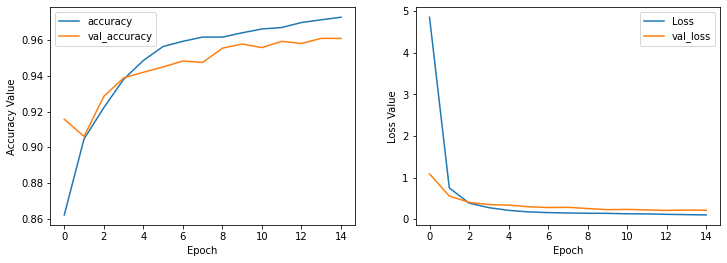
plot_history(history_two_layer)
Creating a three layer network with Fully Connected layer#
input_shape = x_train.shape[1]*x_train.shape[2]
## Implement sequential leyers
model = keras.models.Sequential()
model.add(keras.layers.Dense(128, activation='relu', input_shape=(input_shape,)))
model.add(keras.layers.Dense(64, activation='relu', ))
model.add(keras.layers.Dense(10, activation='softmax'))

model.summary()
Model: "sequential_15"
_________________________________________________________________
 Layer (type)                Output Shape              Param #
=================================================================
 dense_23 (Dense)            (None, 128)               100480

 dense_24 (Dense)            (None, 64)                8256

 dense_25 (Dense)            (None, 10)                650

=================================================================
Total params: 109,386
Trainable params: 109,386
Non-trainable params: 0
_________________________________________________________________
batch_size = 128
epochs = 15

model.compile(loss=["categorical_crossentropy",'mse'], optimizer='adam'
                ,metrics=['accuracy'])

history_three_layer = model.fit(
    x_train_reshaped ,
    y_train_binray_vec,
    batch_size=batch_size,
    epochs=epochs,
    validation_split=0.1
)
Epoch 1/15
422/422 [==============================] - 2s 4ms/step - loss: 2.7456 - accuracy: 0.8495 - val_loss: 0.6261 - val_accuracy: 0.9173
Epoch 2/15
422/422 [==============================] - 1s 3ms/step - loss: 0.4747 - accuracy: 0.9233 - val_loss: 0.3464 - val_accuracy: 0.9427
Epoch 3/15
422/422 [==============================] - 1s 3ms/step - loss: 0.2718 - accuracy: 0.9432 - val_loss: 0.2914 - val_accuracy: 0.9453
Epoch 4/15
422/422 [==============================] - 1s 3ms/step - loss: 0.1903 - accuracy: 0.9556 - val_loss: 0.2557 - val_accuracy: 0.9495
Epoch 5/15
422/422 [==============================] - 1s 4ms/step - loss: 0.1514 - accuracy: 0.9618 - val_loss: 0.2171 - val_accuracy: 0.9575
Epoch 6/15
422/422 [==============================] - 1s 4ms/step - loss: 0.1296 - accuracy: 0.9657 - val_loss: 0.2458 - val_accuracy: 0.9578
Epoch 7/15
422/422 [==============================] - 1s 4ms/step - loss: 0.1150 - accuracy: 0.9697 - val_loss: 0.2395 - val_accuracy: 0.9592
Epoch 8/15
422/422 [==============================] - 1s 4ms/step - loss: 0.1131 - accuracy: 0.9705 - val_loss: 0.2416 - val_accuracy: 0.9555
Epoch 9/15
422/422 [==============================] - 1s 4ms/step - loss: 0.0966 - accuracy: 0.9740 - val_loss: 0.2131 - val_accuracy: 0.9620
Epoch 10/15
422/422 [==============================] - 2s 4ms/step - loss: 0.0880 - accuracy: 0.9754 - val_loss: 0.2323 - val_accuracy: 0.9597
Epoch 11/15
422/422 [==============================] - 2s 4ms/step - loss: 0.0901 - accuracy: 0.9749 - val_loss: 0.2405 - val_accuracy: 0.9527
Epoch 12/15
422/422 [==============================] - 1s 3ms/step - loss: 0.0856 - accuracy: 0.9766 - val_loss: 0.1803 - val_accuracy: 0.9657
Epoch 13/15
422/422 [==============================] - 2s 4ms/step - loss: 0.0718 - accuracy: 0.9800 - val_loss: 0.1925 - val_accuracy: 0.9678
Epoch 14/15
422/422 [==============================] - 2s 4ms/step - loss: 0.0723 - accuracy: 0.9802 - val_loss: 0.1886 - val_accuracy: 0.9673
Epoch 15/15
422/422 [==============================] - 2s 4ms/step - loss: 0.0644 - accuracy: 0.9818 - val_loss: 0.1691 - val_accuracy: 0.9707
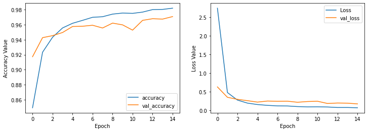
plot_history(history_three_layer)
Let’s see how softmax activation function works in our three layer network.(If we apply softmax function on all the layers)
input_shape = x_train.shape[1]*x_train.shape[2]
## Implement sequential leyers
model = keras.models.Sequential()
model.add(keras.layers.Dense(128, activation='softmax', input_shape=(input_shape,)))
model.add(keras.layers.Dense(64, activation='softmax', ))
model.add(keras.layers.Dense(10, activation='softmax'))

model.summary()
Model: "sequential_16"
_________________________________________________________________
 Layer (type)                Output Shape              Param #
=================================================================
 dense_26 (Dense)            (None, 128)               100480

 dense_27 (Dense)            (None, 64)                8256

 dense_28 (Dense)            (None, 10)                650

=================================================================
Total params: 109,386
Trainable params: 109,386
Non-trainable params: 0
_________________________________________________________________
batch_size = 128
epochs = 15

model.compile(loss=["categorical_crossentropy",'mse'], optimizer='adam'
                ,metrics=['accuracy'])

history_three_layer_softmax_applied = model.fit(
    x_train_reshaped ,
    y_train_binray_vec,
    batch_size=batch_size,
    epochs=epochs,
    validation_split=0.1
)
Epoch 1/15
422/422 [==============================] - 2s 4ms/step - loss: 2.2584 - accuracy: 0.2709 - val_loss: 2.1583 - val_accuracy: 0.6877
Epoch 2/15
422/422 [==============================] - 2s 4ms/step - loss: 1.9198 - accuracy: 0.6935 - val_loss: 1.5972 - val_accuracy: 0.7358
Epoch 3/15
422/422 [==============================] - 2s 4ms/step - loss: 1.3641 - accuracy: 0.7059 - val_loss: 1.0940 - val_accuracy: 0.7348
Epoch 4/15
422/422 [==============================] - 2s 4ms/step - loss: 1.0376 - accuracy: 0.7140 - val_loss: 0.9237 - val_accuracy: 0.7332
Epoch 5/15
422/422 [==============================] - 2s 4ms/step - loss: 0.9187 - accuracy: 0.7205 - val_loss: 0.9217 - val_accuracy: 0.7102
Epoch 6/15
422/422 [==============================] - 2s 4ms/step - loss: 0.8659 - accuracy: 0.7214 - val_loss: 0.8921 - val_accuracy: 0.7103
Epoch 7/15
422/422 [==============================] - 2s 4ms/step - loss: 0.8235 - accuracy: 0.7226 - val_loss: 0.7432 - val_accuracy: 0.7385
Epoch 8/15
422/422 [==============================] - 2s 4ms/step - loss: 0.8051 - accuracy: 0.7259 - val_loss: 0.7229 - val_accuracy: 0.7485
Epoch 9/15
422/422 [==============================] - 2s 4ms/step - loss: 0.7859 - accuracy: 0.7258 - val_loss: 0.7461 - val_accuracy: 0.7443
Epoch 10/15
422/422 [==============================] - 2s 4ms/step - loss: 0.7729 - accuracy: 0.7332 - val_loss: 0.7027 - val_accuracy: 0.7478
Epoch 11/15
422/422 [==============================] - 2s 4ms/step - loss: 0.7674 - accuracy: 0.7362 - val_loss: 0.7341 - val_accuracy: 0.7400
Epoch 12/15
422/422 [==============================] - 2s 4ms/step - loss: 0.7589 - accuracy: 0.7401 - val_loss: 0.7172 - val_accuracy: 0.7553
Epoch 13/15
422/422 [==============================] - 2s 4ms/step - loss: 0.7445 - accuracy: 0.7433 - val_loss: 0.7035 - val_accuracy: 0.7557
Epoch 14/15
422/422 [==============================] - 2s 4ms/step - loss: 0.7277 - accuracy: 0.7406 - val_loss: 0.6770 - val_accuracy: 0.7483
Epoch 15/15
422/422 [==============================] - 2s 4ms/step - loss: 0.7210 - accuracy: 0.7430 - val_loss: 0.6574 - val_accuracy: 0.7598
plot_history(history_three_layer_softmax_applied)
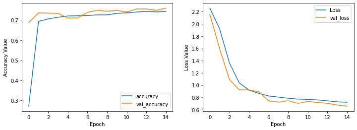
We can see that using the softmax activation function for all layers can achieve much better performance than before, And we can conclude that the softmax activation function can represent and save the pixels information way better than relu.
Let’s apply the tanh activation function for our well behaved three layer network and see the results.
input_shape = x_train.shape[1]*x_train.shape[2]
## Implement sequential leyers
model = keras.models.Sequential()
model.add(keras.layers.Dense(128, activation='tanh', input_shape=(input_shape,)))
model.add(keras.layers.Dense(64, activation='tanh', ))
model.add(keras.layers.Dense(10, activation='tanh'))

model.summary()
Model: "sequential_17"
_________________________________________________________________
 Layer (type)                Output Shape              Param #
=================================================================
 dense_29 (Dense)            (None, 128)               100480

 dense_30 (Dense)            (None, 64)                8256

 dense_31 (Dense)            (None, 10)                650

=================================================================
Total params: 109,386
Trainable params: 109,386
Non-trainable params: 0
_________________________________________________________________
batch_size = 128
epochs = 15

model.compile(loss=["categorical_crossentropy",'mse'], optimizer='adam'
                ,metrics=['accuracy'])

history_three_layer_tanh_applied = model.fit(
    x_train_reshaped ,
    y_train_binray_vec,
    batch_size=batch_size,
    epochs=epochs,
    validation_split=0.1
)
Epoch 1/15
422/422 [==============================] - 2s 4ms/step - loss: 7.9846 - accuracy: 0.1421 - val_loss: 6.6503 - val_accuracy: 0.1108
Epoch 2/15
422/422 [==============================] - 2s 4ms/step - loss: 7.2211 - accuracy: 0.1014 - val_loss: 7.5003 - val_accuracy: 0.1233
Epoch 3/15
422/422 [==============================] - 2s 4ms/step - loss: 7.8166 - accuracy: 0.1290 - val_loss: 7.9597 - val_accuracy: 0.1523
Epoch 4/15
422/422 [==============================] - 2s 4ms/step - loss: 8.1841 - accuracy: 0.1425 - val_loss: 7.9570 - val_accuracy: 0.1528
Epoch 5/15
422/422 [==============================] - 2s 4ms/step - loss: 8.1642 - accuracy: 0.1446 - val_loss: 7.6170 - val_accuracy: 0.1545
Epoch 6/15
422/422 [==============================] - 2s 4ms/step - loss: 7.8573 - accuracy: 0.1026 - val_loss: 7.8253 - val_accuracy: 0.0835
Epoch 7/15
422/422 [==============================] - 2s 4ms/step - loss: 8.0590 - accuracy: 0.0797 - val_loss: 7.8253 - val_accuracy: 0.0835
Epoch 8/15
422/422 [==============================] - 2s 4ms/step - loss: 8.0590 - accuracy: 0.0797 - val_loss: 7.8253 - val_accuracy: 0.0835
Epoch 9/15
422/422 [==============================] - 2s 4ms/step - loss: 8.0590 - accuracy: 0.0797 - val_loss: 7.8253 - val_accuracy: 0.0835
Epoch 10/15
422/422 [==============================] - 2s 4ms/step - loss: 8.0591 - accuracy: 0.0797 - val_loss: 7.8253 - val_accuracy: 0.0835
Epoch 11/15
422/422 [==============================] - 2s 4ms/step - loss: 8.0590 - accuracy: 0.0797 - val_loss: 7.8253 - val_accuracy: 0.0835
Epoch 12/15
422/422 [==============================] - 2s 4ms/step - loss: 8.0590 - accuracy: 0.0797 - val_loss: 7.8253 - val_accuracy: 0.0835
Epoch 13/15
422/422 [==============================] - 2s 4ms/step - loss: 8.0591 - accuracy: 0.0797 - val_loss: 7.8253 - val_accuracy: 0.0835
Epoch 14/15
422/422 [==============================] - 2s 4ms/step - loss: 8.0591 - accuracy: 0.0797 - val_loss: 7.8253 - val_accuracy: 0.0835
Epoch 15/15
422/422 [==============================] - 2s 4ms/step - loss: 8.0591 - accuracy: 0.0797 - val_loss: 7.8253 - val_accuracy: 0.0835
plot_history(history_three_layer_tanh_applied)
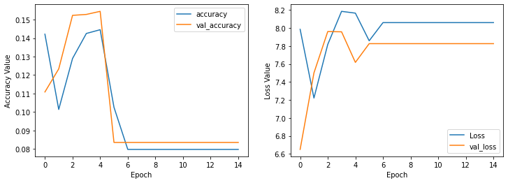
So we could see that the tanh activation function also does not have comparable results to softmax activation function. To have a final result in question 1 we can say that using the softmax activation function can get us to a good accuracy.
Q2#
Question#
Using the imdb dataset try the steps in question 1 and also for tuning try validation dataset.
Answer#
(x_train, y_train), (x_test, y_test) = keras.datasets.imdb.load_data()
First Let’s have a look at the dataset.
x_train.shape
(25000,)
x_train[:2]
array([list([1, 14, 22, 16, 43, 530, 973, 1622, 1385, 65, 458, 4468, 66, 3941, 4, 173, 36, 256, 5, 25, 100, 43, 838, 112, 50, 670, 22665, 9, 35, 480, 284, 5, 150, 4, 172, 112, 167, 21631, 336, 385, 39, 4, 172, 4536, 1111, 17, 546, 38, 13, 447, 4, 192, 50, 16, 6, 147, 2025, 19, 14, 22, 4, 1920, 4613, 469, 4, 22, 71, 87, 12, 16, 43, 530, 38, 76, 15, 13, 1247, 4, 22, 17, 515, 17, 12, 16, 626, 18, 19193, 5, 62, 386, 12, 8, 316, 8, 106, 5, 4, 2223, 5244, 16, 480, 66, 3785, 33, 4, 130, 12, 16, 38, 619, 5, 25, 124, 51, 36, 135, 48, 25, 1415, 33, 6, 22, 12, 215, 28, 77, 52, 5, 14, 407, 16, 82, 10311, 8, 4, 107, 117, 5952, 15, 256, 4, 31050, 7, 3766, 5, 723, 36, 71, 43, 530, 476, 26, 400, 317, 46, 7, 4, 12118, 1029, 13, 104, 88, 4, 381, 15, 297, 98, 32, 2071, 56, 26, 141, 6, 194, 7486, 18, 4, 226, 22, 21, 134, 476, 26, 480, 5, 144, 30, 5535, 18, 51, 36, 28, 224, 92, 25, 104, 4, 226, 65, 16, 38, 1334, 88, 12, 16, 283, 5, 16, 4472, 113, 103, 32, 15, 16, 5345, 19, 178, 32]),
       list([1, 194, 1153, 194, 8255, 78, 228, 5, 6, 1463, 4369, 5012, 134, 26, 4, 715, 8, 118, 1634, 14, 394, 20, 13, 119, 954, 189, 102, 5, 207, 110, 3103, 21, 14, 69, 188, 8, 30, 23, 7, 4, 249, 126, 93, 4, 114, 9, 2300, 1523, 5, 647, 4, 116, 9, 35, 8163, 4, 229, 9, 340, 1322, 4, 118, 9, 4, 130, 4901, 19, 4, 1002, 5, 89, 29, 952, 46, 37, 4, 455, 9, 45, 43, 38, 1543, 1905, 398, 4, 1649, 26, 6853, 5, 163, 11, 3215, 10156, 4, 1153, 9, 194, 775, 7, 8255, 11596, 349, 2637, 148, 605, 15358, 8003, 15, 123, 125, 68, 23141, 6853, 15, 349, 165, 4362, 98, 5, 4, 228, 9, 43, 36893, 1157, 15, 299, 120, 5, 120, 174, 11, 220, 175, 136, 50, 9, 4373, 228, 8255, 5, 25249, 656, 245, 2350, 5, 4, 9837, 131, 152, 491, 18, 46151, 32, 7464, 1212, 14, 9, 6, 371, 78, 22, 625, 64, 1382, 9, 8, 168, 145, 23, 4, 1690, 15, 16, 4, 1355, 5, 28, 6, 52, 154, 462, 33, 89, 78, 285, 16, 145, 95])],
      dtype=object)
## let's see does each item have same length or not
len(x_train[0]), len(x_train[1])
(218, 189)
The description of IMDB datset written in keras docs is as below
This is a dataset of 25,000 movies reviews from IMDB, labeled by sentiment (positive/negative). Reviews have been preprocessed, and each review is encoded as a list of word indexes (integers). For convenience, words are indexed by overall frequency in the dataset, so that for instance the integer "3" encodes the 3rd most frequent word in the data. This allows for quick filtering operations such as: "only consider the top 10,000 most common words, but eliminate the top 20 most common words". As a convention, "0" does not stand for a specific word, but instead is used to encode any unknown word.
So for the EDA step, we will create each sample’s length 2500, in order to have same sample lengths. (because the higest sample length is near 2500, we found it by while coding and got errors)
def modify_dataset(dataset_x, max_length=2500):
    """
    modify each word in dataset by creating a vector for each sample with 1000 length count.

    Parameters:
    -----------
    dataset_x : 2D array
        array of vectors representing each data
    max_length : integer
        max_length of each vector
        default is 1000

    Returns:
    --------
    modified_dataset_x : 2D array
        the modified dataset with the same length of original dataset but having the same length for each item too
    """
    modified_dataset_x = np.zeros((len(dataset_x) , max_length))
    for idx, sample in enumerate(x_train):
        modified_dataset_x[idx][:len(sample)] = sample

    return modified_dataset_x
x_train = modify_dataset(x_train)
x_test = modify_dataset(x_test)

x_train.shape, x_test.shape
((25000, 2500), (25000, 2500))
y_train
array([1, 0, 0, ..., 0, 1, 0], dtype=int64)
It seems that there is no need to categorize the output because the output value for each data is having length one.
to create one layer network because our outputs are length 1, one neuron must be applied, so we’re using two layer network to get better performance. In the first layer we are using 512 neurons with softmax activation function.
because we know in the input each sample size is 2500, we put 2500 nerons in the input layer.
model_imdb = keras.Sequential()
model_imdb.add(keras.layers.Dense(2500, activation='softmax', input_shape=(2500, )))
model_imdb.add(keras.layers.Dense(1, activation='relu', input_shape=(2500, )))


model_imdb.summary()
Model: "sequential_12"
_________________________________________________________________
 Layer (type)                Output Shape              Param #
=================================================================
 dense_16 (Dense)            (None, 2500)              6252500

 dense_17 (Dense)            (None, 1)                 2501

=================================================================
Total params: 6,255,001
Trainable params: 6,255,001
Non-trainable params: 0
_________________________________________________________________
model_imdb.compile(optimizer=tf.keras.optimizers.Adam(learning_rate=1e-3),
              loss=tf.keras.losses.BinaryCrossentropy(),
              metrics=[tf.keras.metrics.BinaryAccuracy(),
                       tf.keras.metrics.FalseNegatives()], )
history_model_imdb = model_imdb.fit(
    x_train ,
    y_train,
    batch_size=32,
    epochs=15,
    validation_split=0.1
)
Epoch 1/15
704/704 [==============================] - 5s 7ms/step - loss: 1.2789 - binary_accuracy: 0.4986 - false_negatives_11: 11281.0000 - val_loss: 0.8314 - val_binary_accuracy: 0.5124 - val_false_negatives_11: 1219.0000
Epoch 2/15
704/704 [==============================] - 5s 7ms/step - loss: 0.7179 - binary_accuracy: 0.4996 - false_negatives_11: 7815.0000 - val_loss: 0.7085 - val_binary_accuracy: 0.4880 - val_false_negatives_11: 27.0000
Epoch 3/15
704/704 [==============================] - 5s 6ms/step - loss: 0.7037 - binary_accuracy: 0.4966 - false_negatives_11: 5514.0000 - val_loss: 0.6981 - val_binary_accuracy: 0.4996 - val_false_negatives_11: 87.0000
Epoch 4/15
704/704 [==============================] - 5s 7ms/step - loss: 0.6954 - binary_accuracy: 0.4994 - false_negatives_11: 3102.0000 - val_loss: 0.6930 - val_binary_accuracy: 0.5124 - val_false_negatives_11: 1219.0000
Epoch 5/15
704/704 [==============================] - 5s 7ms/step - loss: 0.6952 - binary_accuracy: 0.5056 - false_negatives_11: 4567.0000 - val_loss: 0.6932 - val_binary_accuracy: 0.4972 - val_false_negatives_11: 255.0000
Epoch 6/15
704/704 [==============================] - 5s 7ms/step - loss: 0.6941 - binary_accuracy: 0.4995 - false_negatives_11: 3750.0000 - val_loss: 0.6933 - val_binary_accuracy: 0.4876 - val_false_negatives_11: 95.0000
Epoch 7/15
704/704 [==============================] - 5s 7ms/step - loss: 0.6945 - binary_accuracy: 0.5032 - false_negatives_11: 4044.0000 - val_loss: 0.6932 - val_binary_accuracy: 0.4876 - val_false_negatives_11: 20.0000
Epoch 8/15
704/704 [==============================] - 5s 7ms/step - loss: 0.6931 - binary_accuracy: 0.5009 - false_negatives_11: 2555.0000 - val_loss: 0.6930 - val_binary_accuracy: 0.5124 - val_false_negatives_11: 1219.0000
Epoch 9/15
704/704 [==============================] - 5s 7ms/step - loss: 0.6931 - binary_accuracy: 0.4990 - false_negatives_11: 4363.0000 - val_loss: 0.6936 - val_binary_accuracy: 0.4872 - val_false_negatives_11: 10.0000
Epoch 10/15
704/704 [==============================] - 5s 7ms/step - loss: 0.6930 - binary_accuracy: 0.5009 - false_negatives_11: 4554.0000 - val_loss: 0.6939 - val_binary_accuracy: 0.4872 - val_false_negatives_11: 10.0000
Epoch 11/15
704/704 [==============================] - 5s 7ms/step - loss: 0.6930 - binary_accuracy: 0.5013 - false_negatives_11: 3003.0000 - val_loss: 0.6932 - val_binary_accuracy: 0.5124 - val_false_negatives_11: 1219.0000
Epoch 12/15
704/704 [==============================] - 5s 7ms/step - loss: 0.6928 - binary_accuracy: 0.5060 - false_negatives_11: 6394.0000 - val_loss: 0.6950 - val_binary_accuracy: 0.4872 - val_false_negatives_11: 10.0000
Epoch 13/15
704/704 [==============================] - 5s 7ms/step - loss: 0.6929 - binary_accuracy: 0.5033 - false_negatives_11: 2661.0000 - val_loss: 0.6941 - val_binary_accuracy: 0.4872 - val_false_negatives_11: 10.0000
Epoch 14/15
704/704 [==============================] - 5s 7ms/step - loss: 0.6930 - binary_accuracy: 0.5049 - false_negatives_11: 2107.0000 - val_loss: 0.6932 - val_binary_accuracy: 0.5124 - val_false_negatives_11: 1219.0000
Epoch 15/15
704/704 [==============================] - 5s 7ms/step - loss: 0.6930 - binary_accuracy: 0.5029 - false_negatives_11: 4702.0000 - val_loss: 0.6935 - val_binary_accuracy: 0.4872 - val_false_negatives_11: 10.0000
plot_history(history_model_imdb,
             ax1_keys=['binary_accuracy', 'val_binary_accuracy'],
             ax2_keys=['loss', 'val_loss'])
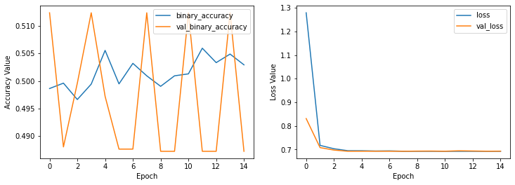
With this values we can easily find out the model is underfitted and is not working properly. So we will try another network with 3 layers to see how the performance change.
model_imdb2 = keras.Sequential()
model_imdb2.add(keras.layers.Dense(2500, activation='softmax', input_shape=(2500, )))
model_imdb2.add(keras.layers.Dense(512, activation='relu', input_shape=(2500, )))
model_imdb2.add(keras.layers.Dense(1, activation='relu', input_shape=(2500, )))


model_imdb2.summary()
Model: "sequential_14"
_________________________________________________________________
 Layer (type)                Output Shape              Param #
=================================================================
 dense_21 (Dense)            (None, 2500)              6252500

 dense_22 (Dense)            (None, 512)               1280512

 dense_23 (Dense)            (None, 1)                 513

=================================================================
Total params: 7,533,525
Trainable params: 7,533,525
Non-trainable params: 0
_________________________________________________________________
model_imdb2.compile(optimizer=tf.keras.optimizers.Adam(learning_rate=1e-3),
              loss=tf.keras.losses.BinaryCrossentropy(),
              metrics=[tf.keras.metrics.BinaryAccuracy(),
                       tf.keras.metrics.FalseNegatives()], )
history_model_imdb2 = model_imdb2.fit(
    x_train ,
    y_train,
    batch_size=32,
    epochs=15,
    validation_split=0.1
)
Epoch 1/15
704/704 [==============================] - 6s 8ms/step - loss: 0.7177 - binary_accuracy: 0.4964 - false_negatives_13: 6128.0000 - val_loss: 0.6927 - val_binary_accuracy: 0.4952 - val_false_negatives_13: 75.0000
Epoch 2/15
704/704 [==============================] - 5s 8ms/step - loss: 0.6962 - binary_accuracy: 0.4943 - false_negatives_13: 5391.0000 - val_loss: 0.6939 - val_binary_accuracy: 0.4852 - val_false_negatives_13: 23.0000
Epoch 3/15
704/704 [==============================] - 6s 8ms/step - loss: 0.6955 - binary_accuracy: 0.4952 - false_negatives_13: 5491.0000 - val_loss: 0.6942 - val_binary_accuracy: 0.4872 - val_false_negatives_13: 36.0000
Epoch 4/15
704/704 [==============================] - 7s 10ms/step - loss: 0.6951 - binary_accuracy: 0.4972 - false_negatives_13: 5806.0000 - val_loss: 0.6926 - val_binary_accuracy: 0.5156 - val_false_negatives_13: 1184.0000
Epoch 5/15
704/704 [==============================] - 6s 8ms/step - loss: 0.6953 - binary_accuracy: 0.4995 - false_negatives_13: 6059.0000 - val_loss: 0.6922 - val_binary_accuracy: 0.4916 - val_false_negatives_13: 6.0000
Epoch 6/15
704/704 [==============================] - 6s 8ms/step - loss: 0.6957 - binary_accuracy: 0.4943 - false_negatives_13: 6224.0000 - val_loss: 0.6947 - val_binary_accuracy: 0.5124 - val_false_negatives_13: 1219.0000
Epoch 7/15
704/704 [==============================] - 6s 8ms/step - loss: 0.6949 - binary_accuracy: 0.5000 - false_negatives_13: 5742.0000 - val_loss: 0.6929 - val_binary_accuracy: 0.5132 - val_false_negatives_13: 1210.0000
Epoch 8/15
704/704 [==============================] - 5s 8ms/step - loss: 0.6950 - binary_accuracy: 0.5067 - false_negatives_13: 5054.0000 - val_loss: 0.6935 - val_binary_accuracy: 0.5088 - val_false_negatives_13: 1188.0000
Epoch 9/15
704/704 [==============================] - 5s 7ms/step - loss: 0.6947 - binary_accuracy: 0.5056 - false_negatives_13: 5765.0000 - val_loss: 0.7007 - val_binary_accuracy: 0.4868 - val_false_negatives_13: 20.0000
Epoch 10/15
704/704 [==============================] - 6s 8ms/step - loss: 0.6949 - binary_accuracy: 0.5020 - false_negatives_13: 5351.0000 - val_loss: 0.7010 - val_binary_accuracy: 0.4876 - val_false_negatives_13: 25.0000
Epoch 11/15
704/704 [==============================] - 5s 7ms/step - loss: 0.6948 - binary_accuracy: 0.4966 - false_negatives_13: 6148.0000 - val_loss: 0.6937 - val_binary_accuracy: 0.4868 - val_false_negatives_13: 24.0000
Epoch 12/15
704/704 [==============================] - 5s 7ms/step - loss: 0.6949 - binary_accuracy: 0.4965 - false_negatives_13: 5391.0000 - val_loss: 0.6934 - val_binary_accuracy: 0.5136 - val_false_negatives_13: 1169.0000
Epoch 13/15
704/704 [==============================] - 5s 7ms/step - loss: 0.6949 - binary_accuracy: 0.4969 - false_negatives_13: 5894.0000 - val_loss: 0.6929 - val_binary_accuracy: 0.5152 - val_false_negatives_13: 1192.0000
Epoch 14/15
704/704 [==============================] - 6s 8ms/step - loss: 0.6946 - binary_accuracy: 0.5016 - false_negatives_13: 5412.0000 - val_loss: 0.6945 - val_binary_accuracy: 0.4860 - val_false_negatives_13: 5.0000
Epoch 15/15
704/704 [==============================] - 5s 8ms/step - loss: 0.6939 - binary_accuracy: 0.5068 - false_negatives_13: 5224.0000 - val_loss: 0.6933 - val_binary_accuracy: 0.4876 - val_false_negatives_13: 5.0000
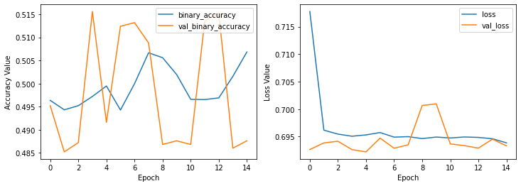
plot_history(history_model_imdb2,
             ax1_keys=['binary_accuracy', 'val_binary_accuracy'],
             ax2_keys=['loss', 'val_loss'])

It seems making a deeper neural network doesn’t work for us. Let’s change relu transfer function, maybe we’re losing information because of choosing wrong activation function.
model_imdb3 = keras.Sequential()
model_imdb3.add(keras.layers.Dense(2500, activation='softmax', input_shape=(2500, )))
model_imdb3.add(keras.layers.Dense(512, activation='softmax', input_shape=(2500, )))
model_imdb3.add(keras.layers.Dense(1, activation='softmax', input_shape=(2500, )))


model_imdb3.summary()
Model: "sequential_16"
_________________________________________________________________
 Layer (type)                Output Shape              Param #
=================================================================
 dense_27 (Dense)            (None, 2500)              6252500

 dense_28 (Dense)            (None, 512)               1280512

 dense_29 (Dense)            (None, 1)                 513

=================================================================
Total params: 7,533,525
Trainable params: 7,533,525
Non-trainable params: 0
_________________________________________________________________
model_imdb3.compile(optimizer=tf.keras.optimizers.Adam(learning_rate=1e-3),
              loss=tf.keras.losses.BinaryCrossentropy(),
              metrics=[tf.keras.metrics.BinaryAccuracy(),
                       tf.keras.metrics.FalseNegatives()], )
history_model_imdb3 = model_imdb3.fit(
    x_train ,
    y_train,
    batch_size=32,
    epochs=15,
    validation_split=0.1
)
Epoch 1/15
704/704 [==============================] - 6s 8ms/step - loss: 0.6931 - binary_accuracy: 0.5014 - false_negatives_14: 0.0000e+00 - val_loss: 0.6931 - val_binary_accuracy: 0.4876 - val_false_negatives_14: 0.0000e+00
Epoch 2/15
704/704 [==============================] - 5s 8ms/step - loss: 0.6932 - binary_accuracy: 0.5014 - false_negatives_14: 0.0000e+00 - val_loss: 0.6938 - val_binary_accuracy: 0.4876 - val_false_negatives_14: 0.0000e+00
Epoch 3/15
704/704 [==============================] - 5s 8ms/step - loss: 0.6932 - binary_accuracy: 0.5014 - false_negatives_14: 0.0000e+00 - val_loss: 0.6929 - val_binary_accuracy: 0.4876 - val_false_negatives_14: 0.0000e+00
Epoch 4/15
704/704 [==============================] - 5s 8ms/step - loss: 0.6932 - binary_accuracy: 0.5014 - false_negatives_14: 0.0000e+00 - val_loss: 0.6935 - val_binary_accuracy: 0.4876 - val_false_negatives_14: 0.0000e+00
Epoch 5/15
704/704 [==============================] - 5s 8ms/step - loss: 0.6932 - binary_accuracy: 0.5014 - false_negatives_14: 0.0000e+00 - val_loss: 0.6929 - val_binary_accuracy: 0.4876 - val_false_negatives_14: 0.0000e+00
Epoch 6/15
704/704 [==============================] - 5s 8ms/step - loss: 0.6932 - binary_accuracy: 0.5014 - false_negatives_14: 0.0000e+00 - val_loss: 0.6933 - val_binary_accuracy: 0.4876 - val_false_negatives_14: 0.0000e+00
Epoch 7/15
704/704 [==============================] - 5s 8ms/step - loss: 0.6932 - binary_accuracy: 0.5014 - false_negatives_14: 0.0000e+00 - val_loss: 0.6933 - val_binary_accuracy: 0.4876 - val_false_negatives_14: 0.0000e+00
Epoch 8/15
704/704 [==============================] - 5s 7ms/step - loss: 0.6932 - binary_accuracy: 0.5014 - false_negatives_14: 0.0000e+00 - val_loss: 0.6933 - val_binary_accuracy: 0.4876 - val_false_negatives_14: 0.0000e+00
Epoch 9/15
704/704 [==============================] - 5s 7ms/step - loss: 0.6932 - binary_accuracy: 0.5014 - false_negatives_14: 0.0000e+00 - val_loss: 0.6932 - val_binary_accuracy: 0.4876 - val_false_negatives_14: 0.0000e+00
Epoch 10/15
704/704 [==============================] - 5s 8ms/step - loss: 0.6932 - binary_accuracy: 0.5014 - false_negatives_14: 0.0000e+00 - val_loss: 0.6930 - val_binary_accuracy: 0.4876 - val_false_negatives_14: 0.0000e+00
Epoch 11/15
704/704 [==============================] - 5s 7ms/step - loss: 0.6932 - binary_accuracy: 0.5014 - false_negatives_14: 0.0000e+00 - val_loss: 0.6931 - val_binary_accuracy: 0.4876 - val_false_negatives_14: 0.0000e+00
Epoch 12/15
704/704 [==============================] - 5s 7ms/step - loss: 0.6932 - binary_accuracy: 0.5014 - false_negatives_14: 0.0000e+00 - val_loss: 0.6932 - val_binary_accuracy: 0.4876 - val_false_negatives_14: 0.0000e+00
Epoch 13/15
704/704 [==============================] - 5s 7ms/step - loss: 0.6932 - binary_accuracy: 0.5014 - false_negatives_14: 0.0000e+00 - val_loss: 0.6938 - val_binary_accuracy: 0.4876 - val_false_negatives_14: 0.0000e+00
Epoch 14/15
704/704 [==============================] - 5s 7ms/step - loss: 0.6932 - binary_accuracy: 0.5014 - false_negatives_14: 0.0000e+00 - val_loss: 0.6930 - val_binary_accuracy: 0.4876 - val_false_negatives_14: 0.0000e+00
Epoch 15/15
704/704 [==============================] - 5s 7ms/step - loss: 0.6932 - binary_accuracy: 0.5014 - false_negatives_14: 0.0000e+00 - val_loss: 0.6931 - val_binary_accuracy: 0.4876 - val_false_negatives_14: 0.0000e+00
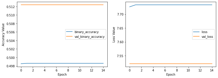
plot_history(history_model_imdb2,
             ax1_keys=['binary_accuracy', 'val_binary_accuracy'],
             ax2_keys=['loss', 'val_loss'])
Again it doesn’t work changing the activation functions. Let’s create a deeper network with different neurons count.
model_imdb4 = keras.Sequential()
model_imdb4.add(keras.layers.Dense(2500, activation='softmax', input_shape=(2500, )))
model_imdb4.add(keras.layers.Dense(1024, activation='relu', input_shape=(2500, )))
model_imdb4.add(keras.layers.Dense(512, activation='relu', input_shape=(2500, )))
model_imdb4.add(keras.layers.Dense(256, activation='relu', input_shape=(2500, )))
model_imdb4.add(keras.layers.Dense(128, activation='relu', input_shape=(2500, )))
model_imdb4.add(keras.layers.Dense(1, activation='relu', input_shape=(2500, )))


model_imdb4.summary()
Model: "sequential_18"
_________________________________________________________________
 Layer (type)                Output Shape              Param #
=================================================================
 dense_36 (Dense)            (None, 2500)              6252500

 dense_37 (Dense)            (None, 1024)              2561024

 dense_38 (Dense)            (None, 512)               524800

 dense_39 (Dense)            (None, 256)               131328

 dense_40 (Dense)            (None, 128)               32896

 dense_41 (Dense)            (None, 1)                 129

=================================================================
Total params: 9,502,677
Trainable params: 9,502,677
Non-trainable params: 0
_________________________________________________________________
## Let's have a high learning rate to see how good it can perform in low count iterations
## having high learning rate can cause to near random results and we want that to see how good it can perform
model_imdb4.compile(optimizer=tf.keras.optimizers.Adam(learning_rate=1e-1),
              loss=tf.keras.losses.BinaryCrossentropy(),
              metrics=[tf.keras.metrics.BinaryAccuracy(),
                       tf.keras.metrics.FalseNegatives()], )
history_model_imdb4 = model_imdb4.fit(
    x_train ,
    y_train,
    batch_size=32,
    epochs=15,
    validation_split=0.1
)
Epoch 1/15
704/704 [==============================] - 7s 9ms/step - loss: 7.7265 - binary_accuracy: 0.4985 - false_negatives_20: 11279.0000 - val_loss: 7.5212 - val_binary_accuracy: 0.5124 - val_false_negatives_20: 1219.0000
Epoch 2/15
704/704 [==============================] - 6s 9ms/step - loss: 7.7337 - binary_accuracy: 0.4986 - false_negatives_20: 11281.0000 - val_loss: 7.5212 - val_binary_accuracy: 0.5124 - val_false_negatives_20: 1219.0000
Epoch 3/15
704/704 [==============================] - 6s 9ms/step - loss: 7.7337 - binary_accuracy: 0.4986 - false_negatives_20: 11281.0000 - val_loss: 7.5212 - val_binary_accuracy: 0.5124 - val_false_negatives_20: 1219.0000
Epoch 4/15
704/704 [==============================] - 6s 9ms/step - loss: 7.7337 - binary_accuracy: 0.4986 - false_negatives_20: 11281.0000 - val_loss: 7.5212 - val_binary_accuracy: 0.5124 - val_false_negatives_20: 1219.0000
Epoch 5/15
704/704 [==============================] - 6s 9ms/step - loss: 7.7337 - binary_accuracy: 0.4986 - false_negatives_20: 11281.0000 - val_loss: 7.5212 - val_binary_accuracy: 0.5124 - val_false_negatives_20: 1219.0000
Epoch 6/15
704/704 [==============================] - 6s 9ms/step - loss: 7.7337 - binary_accuracy: 0.4986 - false_negatives_20: 11281.0000 - val_loss: 7.5212 - val_binary_accuracy: 0.5124 - val_false_negatives_20: 1219.0000
Epoch 7/15
704/704 [==============================] - 6s 9ms/step - loss: 7.7337 - binary_accuracy: 0.4986 - false_negatives_20: 11281.0000 - val_loss: 7.5212 - val_binary_accuracy: 0.5124 - val_false_negatives_20: 1219.0000
Epoch 8/15
704/704 [==============================] - 6s 9ms/step - loss: 7.7337 - binary_accuracy: 0.4986 - false_negatives_20: 11281.0000 - val_loss: 7.5212 - val_binary_accuracy: 0.5124 - val_false_negatives_20: 1219.0000
Epoch 9/15
704/704 [==============================] - 6s 9ms/step - loss: 7.7337 - binary_accuracy: 0.4986 - false_negatives_20: 11281.0000 - val_loss: 7.5212 - val_binary_accuracy: 0.5124 - val_false_negatives_20: 1219.0000
Epoch 10/15
704/704 [==============================] - 6s 9ms/step - loss: 7.7337 - binary_accuracy: 0.4986 - false_negatives_20: 11281.0000 - val_loss: 7.5212 - val_binary_accuracy: 0.5124 - val_false_negatives_20: 1219.0000
Epoch 11/15
704/704 [==============================] - 6s 9ms/step - loss: 7.7337 - binary_accuracy: 0.4986 - false_negatives_20: 11281.0000 - val_loss: 7.5212 - val_binary_accuracy: 0.5124 - val_false_negatives_20: 1219.0000
Epoch 12/15
704/704 [==============================] - 6s 9ms/step - loss: 7.7337 - binary_accuracy: 0.4986 - false_negatives_20: 11281.0000 - val_loss: 7.5212 - val_binary_accuracy: 0.5124 - val_false_negatives_20: 1219.0000
Epoch 13/15
704/704 [==============================] - 6s 9ms/step - loss: 7.7337 - binary_accuracy: 0.4986 - false_negatives_20: 11281.0000 - val_loss: 7.5212 - val_binary_accuracy: 0.5124 - val_false_negatives_20: 1219.0000
Epoch 14/15
704/704 [==============================] - 6s 9ms/step - loss: 7.7337 - binary_accuracy: 0.4986 - false_negatives_20: 11281.0000 - val_loss: 7.5212 - val_binary_accuracy: 0.5124 - val_false_negatives_20: 1219.0000
Epoch 15/15
704/704 [==============================] - 6s 9ms/step - loss: 7.7337 - binary_accuracy: 0.4986 - false_negatives_20: 11281.0000 - val_loss: 7.5212 - val_binary_accuracy: 0.5124 - val_false_negatives_20: 1219.0000
plot_history(history_model_imdb4,
             ax1_keys=['binary_accuracy', 'val_binary_accuracy'],
             ax2_keys=['loss', 'val_loss'])
It is not performing well again! So we need to use other layer types to achieve better performance.
Maybe categorizing the output values can help us to get a better performance. Because the output values was length one we had to force the output layer to have one neuron and categorizing it can create two values for each output (So we set output nurons to 2).
y_train_categorized = keras.utils.to_categorical(y_train)
y_test_categorized = keras.utils.to_categorical(y_test)
model_imdb5 = keras.Sequential()
model_imdb5.add(keras.layers.Dense(2500, activation='softmax', input_shape=(2500, )))
model_imdb5.add(keras.layers.Dense(1024, activation='relu', input_shape=(2500, )))
model_imdb5.add(keras.layers.Dense(512, activation='relu', input_shape=(2500, )))
model_imdb5.add(keras.layers.Dense(256, activation='relu', input_shape=(2500, )))
model_imdb5.add(keras.layers.Dense(128, activation='relu', input_shape=(2500, )))
model_imdb5.add(keras.layers.Dense(2, activation='relu', input_shape=(2500, )))


model_imdb5.compile(optimizer=tf.keras.optimizers.Adam(learning_rate=1e-3),
              loss=tf.keras.losses.BinaryCrossentropy(),
              metrics=[tf.keras.metrics.BinaryAccuracy(),
                       tf.keras.metrics.FalseNegatives()], )

history_model_imdb5 = model_imdb5.fit(
    x_train,
    y_train_categorized,
    batch_size=32,
    epochs=15,
    validation_split=0.1
)
Epoch 1/15
704/704 [==============================] - 7s 9ms/step - loss: 4.2024 - binary_accuracy: 0.4999 - false_negatives_24: 17616.0000 - val_loss: 4.3118 - val_binary_accuracy: 0.4876 - val_false_negatives_24: 1283.0000
Epoch 2/15
704/704 [==============================] - 6s 9ms/step - loss: 4.1946 - binary_accuracy: 0.4986 - false_negatives_24: 17285.0000 - val_loss: 4.2982 - val_binary_accuracy: 0.5012 - val_false_negatives_24: 2476.0000
Epoch 3/15
704/704 [==============================] - 6s 9ms/step - loss: 4.1943 - binary_accuracy: 0.4990 - false_negatives_24: 17456.0000 - val_loss: 4.2999 - val_binary_accuracy: 0.4876 - val_false_negatives_24: 1281.0000
Epoch 4/15
704/704 [==============================] - 6s 9ms/step - loss: 4.1930 - binary_accuracy: 0.5030 - false_negatives_24: 16756.0000 - val_loss: 4.2983 - val_binary_accuracy: 0.5006 - val_false_negatives_24: 2483.0000
Epoch 5/15
704/704 [==============================] - 6s 9ms/step - loss: 4.1929 - binary_accuracy: 0.5004 - false_negatives_24: 16507.0000 - val_loss: 4.3005 - val_binary_accuracy: 0.4876 - val_false_negatives_24: 1281.0000
Epoch 6/15
704/704 [==============================] - 6s 9ms/step - loss: 4.1928 - binary_accuracy: 0.5016 - false_negatives_24: 17048.0000 - val_loss: 4.3007 - val_binary_accuracy: 0.4876 - val_false_negatives_24: 1281.0000
Epoch 7/15
704/704 [==============================] - 6s 9ms/step - loss: 4.1931 - binary_accuracy: 0.4978 - false_negatives_24: 17008.0000 - val_loss: 4.2983 - val_binary_accuracy: 0.5000 - val_false_negatives_24: 2500.0000
Epoch 8/15
704/704 [==============================] - 6s 9ms/step - loss: 4.1928 - binary_accuracy: 0.4996 - false_negatives_24: 17103.0000 - val_loss: 4.2987 - val_binary_accuracy: 0.4878 - val_false_negatives_24: 1281.0000
Epoch 9/15
704/704 [==============================] - 6s 9ms/step - loss: 4.1927 - binary_accuracy: 0.5022 - false_negatives_24: 16023.0000 - val_loss: 4.2989 - val_binary_accuracy: 0.4878 - val_false_negatives_24: 1281.0000
Epoch 10/15
704/704 [==============================] - 6s 9ms/step - loss: 4.1931 - binary_accuracy: 0.4985 - false_negatives_24: 16556.0000 - val_loss: 4.2985 - val_binary_accuracy: 0.4882 - val_false_negatives_24: 1282.0000
Epoch 11/15
704/704 [==============================] - 6s 9ms/step - loss: 4.1931 - binary_accuracy: 0.4995 - false_negatives_24: 17002.0000 - val_loss: 4.2992 - val_binary_accuracy: 0.4876 - val_false_negatives_24: 1281.0000
Epoch 12/15
704/704 [==============================] - 7s 9ms/step - loss: 4.1945 - binary_accuracy: 0.5005 - false_negatives_24: 16570.0000 - val_loss: 4.2982 - val_binary_accuracy: 0.5000 - val_false_negatives_24: 2500.0000
Epoch 13/15
704/704 [==============================] - 7s 9ms/step - loss: 4.1942 - binary_accuracy: 0.4992 - false_negatives_24: 16712.0000 - val_loss: 4.2986 - val_binary_accuracy: 0.4874 - val_false_negatives_24: 1282.0000
Epoch 14/15
704/704 [==============================] - 6s 9ms/step - loss: 4.1925 - binary_accuracy: 0.5028 - false_negatives_24: 16595.0000 - val_loss: 4.3005 - val_binary_accuracy: 0.4876 - val_false_negatives_24: 1281.0000
Epoch 15/15
704/704 [==============================] - 6s 9ms/step - loss: 4.1926 - binary_accuracy: 0.4984 - false_negatives_24: 17000.0000 - val_loss: 4.2986 - val_binary_accuracy: 0.5000 - val_false_negatives_24: 2500.0000
Until now we tried a lot to get a good performance with dense layers in imdb dataset, but it seems this kind of networks cannot perform well in this situation and we must try other leyers (Here the dense layers can is performing as good as a random classifier).
The code above is a use of the example of tensorflow toturials to help us how to create better model using text embeding (https://www.tensorflow.org/tutorials/keras/text_classification_with_hub).
## downloading another version of IMDB dataset
## in this version the texts are available
train_data, validation_data, test_data = tfds.load(
    name="imdb_reviews",
    split=('train[:60%]', 'train[60%:]', 'test'),
    as_supervised=True)
train_examples_batch, train_labels_batch = next(iter(train_data.batch(5)))
train_examples_batch
<tf.Tensor: shape=(5,), dtype=string, numpy=
array([b"This was an absolutely terrible movie. Don't be lured in by Christopher Walken or Michael Ironside. Both are great actors, but this must simply be their worst role in history. Even their great acting could not redeem this movie's ridiculous storyline. This movie is an early nineties US propaganda piece. The most pathetic scenes were those when the Columbian rebels were making their cases for revolutions. Maria Conchita Alonso appeared phony, and her pseudo-love affair with Walken was nothing but a pathetic emotional plug in a movie that was devoid of any real meaning. I am disappointed that there are movies like this, ruining actor's like Christopher Walken's good name. I could barely sit through it.",
       b'I have been known to fall asleep during films, but this is usually due to a combination of things including, really tired, being warm and comfortable on the sette and having just eaten a lot. However on this occasion I fell asleep because the film was rubbish. The plot development was constant. Constantly slow and boring. Things seemed to happen, but with no explanation of what was causing them or why. I admit, I may have missed part of the film, but i watched the majority of it and everything just seemed to happen of its own accord without any real concern for anything else. I cant recommend this film at all.',
       b'Mann photographs the Alberta Rocky Mountains in a superb fashion, and Jimmy Stewart and Walter Brennan give enjoyable performances as they always seem to do. <br /><br />But come on Hollywood - a Mountie telling the people of Dawson City, Yukon to elect themselves a marshal (yes a marshal!) and to enforce the law themselves, then gunfighters battling it out on the streets for control of the town? <br /><br />Nothing even remotely resembling that happened on the Canadian side of the border during the Klondike gold rush. Mr. Mann and company appear to have mistaken Dawson City for Deadwood, the Canadian North for the American Wild West.<br /><br />Canadian viewers be prepared for a Reefer Madness type of enjoyable howl with this ludicrous plot, or, to shake your head in disgust.',
       b'This is the kind of film for a snowy Sunday afternoon when the rest of the world can go ahead with its own business as you descend into a big arm-chair and mellow for a couple of hours. Wonderful performances from Cher and Nicolas Cage (as always) gently row the plot along. There are no rapids to cross, no dangerous waters, just a warm and witty paddle through New York life at its best. A family film in every sense and one that deserves the praise it received.',
       b'As others have mentioned, all the women that go nude in this film are mostly absolutely gorgeous. The plot very ably shows the hypocrisy of the female libido. When men are around they want to be pursued, but when no "men" are around, they become the pursuers of a 14 year old boy. And the boy becomes a man really fast (we should all be so lucky at this age!). He then gets up the courage to pursue his true love.'],
      dtype=object)>
train_labels_batch
<tf.Tensor: shape=(5,), dtype=int64, numpy=array([0, 0, 0, 1, 1], dtype=int64)>
We will use a pre-defined text embeding model from TFHub:”https://tfhub.dev/google/nnlm-en-dim50/2”
embedding = "https://tfhub.dev/google/nnlm-en-dim50/2"
hub_layer = hub.KerasLayer(embedding, input_shape=[],
                           dtype=tf.string, trainable=True)
hub_layer(train_examples_batch[:3])
<tf.Tensor: shape=(3, 50), dtype=float32, numpy=
array([[ 0.5423195 , -0.0119017 ,  0.06337538,  0.06862972, -0.16776837,
        -0.10581174,  0.16865303, -0.04998824, -0.31148055,  0.07910346,
         0.15442263,  0.01488662,  0.03930153,  0.19772711, -0.12215476,
        -0.04120981, -0.2704109 , -0.21922152,  0.26517662, -0.80739075,
         0.25833532, -0.3100421 ,  0.28683215,  0.1943387 , -0.29036492,
         0.03862849, -0.7844411 , -0.0479324 ,  0.4110299 , -0.36388892,
        -0.58034706,  0.30269456,  0.3630897 , -0.15227164, -0.44391504,
         0.19462997,  0.19528408,  0.05666234,  0.2890704 , -0.28468323,
        -0.00531206,  0.0571938 , -0.3201318 , -0.04418665, -0.08550783,
        -0.55847436, -0.23336391, -0.20782952, -0.03543064, -0.17533456],
       [ 0.56338924, -0.12339553, -0.10862679,  0.7753425 , -0.07667089,
        -0.15752277,  0.01872335, -0.08169781, -0.3521876 ,  0.4637341 ,
        -0.08492756,  0.07166859, -0.00670817,  0.12686075, -0.19326553,
        -0.52626437, -0.3295823 ,  0.14394785,  0.09043556, -0.5417555 ,
         0.02468163, -0.15456742,  0.68333143,  0.09068331, -0.45327246,
         0.23180096, -0.8615696 ,  0.34480393,  0.12838456, -0.58759046,
        -0.4071231 ,  0.23061076,  0.48426893, -0.27128142, -0.5380916 ,
         0.47016326,  0.22572741, -0.00830663,  0.2846242 , -0.304985  ,
         0.04400365,  0.25025874,  0.14867121,  0.40717036, -0.15422426,
        -0.06878027, -0.40825695, -0.3149215 ,  0.09283665, -0.20183425],
       [ 0.7456154 ,  0.21256861,  0.14400336,  0.5233862 ,  0.11032254,
         0.00902788, -0.3667802 , -0.08938274, -0.24165542,  0.33384594,
        -0.11194605, -0.01460047, -0.0071645 ,  0.19562712,  0.00685216,
        -0.24886718, -0.42796347,  0.18620004, -0.05241098, -0.66462487,
         0.13449019, -0.22205497,  0.08633006,  0.43685386,  0.2972681 ,
         0.36140734, -0.7196889 ,  0.05291241, -0.14316116, -0.1573394 ,
        -0.15056328, -0.05988009, -0.08178931, -0.15569411, -0.09303783,
        -0.18971172,  0.07620788, -0.02541647, -0.27134508, -0.3392682 ,
        -0.10296468, -0.27275252, -0.34078008,  0.20083304, -0.26644835,
         0.00655449, -0.05141488, -0.04261917, -0.45413622,  0.20023568]],
      dtype=float32)>
model_imdb_tfhub = tf.keras.Sequential()
model_imdb_tfhub.add(hub_layer)
model_imdb_tfhub.add(tf.keras.layers.Dense(16, activation='relu'))
model_imdb_tfhub.add(tf.keras.layers.Dense(1))

model_imdb_tfhub.summary()
Model: "sequential"
_________________________________________________________________
 Layer (type)                Output Shape              Param #
=================================================================
 keras_layer (KerasLayer)    (None, 50)                48190600

 dense (Dense)               (None, 16)                816

 dense_1 (Dense)             (None, 1)                 17

=================================================================
Total params: 48,191,433
Trainable params: 48,191,433
Non-trainable params: 0
_________________________________________________________________
model_imdb_tfhub.compile(optimizer='adam',
              loss=tf.keras.losses.BinaryCrossentropy(from_logits=True),
              metrics=['accuracy', 'mse'])

history_imdb_tfhub = model_imdb_tfhub.fit(train_data.shuffle(10000).batch(512),
                    epochs=15,
                    validation_data=validation_data.batch(512),
                    verbose=1)
Epoch 1/15
30/30 [==============================] - 2s 63ms/step - loss: 0.0386 - accuracy: 0.9937 - mse: 27.3006 - val_loss: 0.3468 - val_accuracy: 0.8688 - val_mse: 24.4022
Epoch 2/15
30/30 [==============================] - 2s 60ms/step - loss: 0.0237 - accuracy: 0.9978 - mse: 34.7808 - val_loss: 0.3680 - val_accuracy: 0.8672 - val_mse: 30.1637
Epoch 3/15
30/30 [==============================] - 2s 59ms/step - loss: 0.0158 - accuracy: 0.9989 - mse: 42.3120 - val_loss: 0.3907 - val_accuracy: 0.8648 - val_mse: 35.5622
Epoch 4/15
30/30 [==============================] - 2s 60ms/step - loss: 0.0104 - accuracy: 0.9995 - mse: 49.2255 - val_loss: 0.4137 - val_accuracy: 0.8671 - val_mse: 40.5303
Epoch 5/15
30/30 [==============================] - 2s 60ms/step - loss: 0.0072 - accuracy: 0.9997 - mse: 56.1228 - val_loss: 0.4302 - val_accuracy: 0.8635 - val_mse: 45.5260
Epoch 6/15
30/30 [==============================] - 2s 60ms/step - loss: 0.0053 - accuracy: 0.9999 - mse: 62.4211 - val_loss: 0.4480 - val_accuracy: 0.8641 - val_mse: 50.0269
Epoch 7/15
30/30 [==============================] - 2s 59ms/step - loss: 0.0040 - accuracy: 0.9999 - mse: 68.1974 - val_loss: 0.4650 - val_accuracy: 0.8660 - val_mse: 54.0439
Epoch 8/15
30/30 [==============================] - 2s 60ms/step - loss: 0.0031 - accuracy: 0.9999 - mse: 73.5167 - val_loss: 0.4791 - val_accuracy: 0.8638 - val_mse: 57.9952
Epoch 9/15
30/30 [==============================] - 2s 60ms/step - loss: 0.0024 - accuracy: 0.9999 - mse: 78.7963 - val_loss: 0.4939 - val_accuracy: 0.8645 - val_mse: 61.8141
Epoch 10/15
30/30 [==============================] - 2s 59ms/step - loss: 0.0019 - accuracy: 1.0000 - mse: 83.6937 - val_loss: 0.5053 - val_accuracy: 0.8636 - val_mse: 65.3866
Epoch 11/15
30/30 [==============================] - 2s 59ms/step - loss: 0.0016 - accuracy: 1.0000 - mse: 88.6348 - val_loss: 0.5190 - val_accuracy: 0.8632 - val_mse: 69.5248
Epoch 12/15
30/30 [==============================] - 2s 60ms/step - loss: 0.0013 - accuracy: 1.0000 - mse: 95.0916 - val_loss: 0.5348 - val_accuracy: 0.8629 - val_mse: 74.7366
Epoch 13/15
30/30 [==============================] - 2s 61ms/step - loss: 0.0010 - accuracy: 1.0000 - mse: 101.8503 - val_loss: 0.5511 - val_accuracy: 0.8619 - val_mse: 79.5027
Epoch 14/15
30/30 [==============================] - 2s 61ms/step - loss: 8.1029e-04 - accuracy: 1.0000 - mse: 108.2622 - val_loss: 0.5644 - val_accuracy: 0.8615 - val_mse: 84.5848
Epoch 15/15
30/30 [==============================] - 2s 60ms/step - loss: 6.6532e-04 - accuracy: 1.0000 - mse: 114.5061 - val_loss: 0.5778 - val_accuracy: 0.8609 - val_mse: 89.0296
plot_history(history_imdb_tfhub)
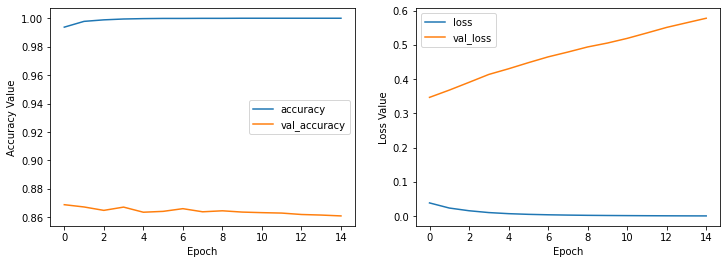
It seems using the text embeding model can help us achieve greate performance. So for text data we can say that using a text embeding model that converts strings to numeric data is a good way to create simple neural networks with few layers. (We just used two layers here and we got near 87 percent accuracy on validation dataset!)
To speak about the last model history we can say that achieving higher accuracy for train data in last iterations moved us to overfit state that it can easily seen in loss diagram.
After getting a good accuracy let’s look at the performance of the model on test data.
results = model_imdb_tfhub.evaluate(test_data.batch(512), verbose=2)

for name, value in zip(model_imdb_tfhub.metrics_names, results):
    print("%s: %.3f" % (name, value))
49/49 - 1s - loss: 0.6359 - accuracy: 0.8429 - mse: 80.1773 - 1s/epoch - 26ms/step
loss: 0.636
accuracy: 0.843
mse: 80.177
So having about 84 percent accuracy for test data is a great performance comparing to the previous results.
Q3#
Part a#
Using CFAR10 dataset, create a convolution network and find the accuracy results.
## to download the dataset we need to renew the ssl certificates
import ssl

ssl._create_default_https_context = ssl._create_unverified_context
(x_train_cifar, y_train_cifar), (x_test_cifar, y_test_cifar) = keras.datasets.cifar10.load_data()
assert x_train_cifar.shape == (50000, 32, 32, 3)
assert x_test_cifar.shape == (10000, 32, 32, 3)
assert y_train_cifar.shape == (50000, 1)
assert y_test_cifar.shape == (10000, 1)
## lets see how many class we have and then we need to specify the output neurons with the length of unique labels
np.unique(y_train_cifar)
array([0, 1, 2, 3, 4, 5, 6, 7, 8, 9], dtype=uint8)
y_train_categorical_cifar = keras.utils.to_categorical(y_train_cifar)
y_test_cifar_categorical_cifar = keras.utils.to_categorical(y_test_cifar)
## normalize data
x_train_cifar = x_train_cifar / 255.0
x_test_cifar = x_test_cifar / 255.0
model_cfar = tf.keras.Sequential()
model_cfar.add(keras.layers.Conv2D(filters=32, input_shape=(32, 32, 3),  kernel_size=(3,3), activation='relu'))
model_cfar.add(keras.layers.MaxPooling2D(pool_size=(2, 2), padding="valid"))
model_cfar.add(keras.layers.Dense(64, activation='softmax'))
model_cfar.add(keras.layers.Flatten())
model_cfar.add(keras.layers.Dense(10, activation='softmax'))

model_cfar.summary()
Model: "sequential_1"
_________________________________________________________________
 Layer (type)                Output Shape              Param #
=================================================================
 conv2d_1 (Conv2D)           (None, 30, 30, 32)        896

 max_pooling2d_1 (MaxPooling  (None, 15, 15, 32)       0
 2D)

 dense_2 (Dense)             (None, 15, 15, 64)        2112

 flatten_1 (Flatten)         (None, 14400)             0

 dense_3 (Dense)             (None, 10)                144010

=================================================================
Total params: 147,018
Trainable params: 147,018
Non-trainable params: 0
_________________________________________________________________
model_cfar.compile(
    optimizer=keras.optimizers.Adam(),
    metrics=['accuracy'] ,
    loss=tf.keras.losses.categorical_crossentropy,
)

history_cifar = model_cfar.fit(x_train_cifar,
               y_train_categorical_cifar,
               epochs=25,
               validation_split=0.1,
               shuffle=True,
               batch_size=32
)
Epoch 1/25
1407/1407 [==============================] - 8s 5ms/step - loss: 0.7979 - accuracy: 0.7249 - val_loss: 1.1035 - val_accuracy: 0.6348
Epoch 2/25
1407/1407 [==============================] - 7s 5ms/step - loss: 0.7598 - accuracy: 0.7380 - val_loss: 1.0906 - val_accuracy: 0.6330
Epoch 3/25
1407/1407 [==============================] - 7s 5ms/step - loss: 0.7244 - accuracy: 0.7525 - val_loss: 1.1206 - val_accuracy: 0.6242
Epoch 4/25
1407/1407 [==============================] - 7s 5ms/step - loss: 0.6911 - accuracy: 0.7636 - val_loss: 1.1183 - val_accuracy: 0.6314
Epoch 5/25
1407/1407 [==============================] - 7s 5ms/step - loss: 0.6550 - accuracy: 0.7776 - val_loss: 1.1160 - val_accuracy: 0.6360
Epoch 6/25
1407/1407 [==============================] - 7s 5ms/step - loss: 0.6203 - accuracy: 0.7904 - val_loss: 1.1572 - val_accuracy: 0.6256
Epoch 7/25
1407/1407 [==============================] - 8s 5ms/step - loss: 0.5840 - accuracy: 0.8052 - val_loss: 1.1693 - val_accuracy: 0.6242
Epoch 8/25
1407/1407 [==============================] - 8s 5ms/step - loss: 0.5499 - accuracy: 0.8182 - val_loss: 1.1754 - val_accuracy: 0.6254
Epoch 9/25
1407/1407 [==============================] - 8s 5ms/step - loss: 0.5134 - accuracy: 0.8332 - val_loss: 1.2162 - val_accuracy: 0.6152
Epoch 10/25
1407/1407 [==============================] - 8s 5ms/step - loss: 0.4805 - accuracy: 0.8441 - val_loss: 1.2524 - val_accuracy: 0.6098
Epoch 11/25
1407/1407 [==============================] - 8s 6ms/step - loss: 0.4453 - accuracy: 0.8595 - val_loss: 1.2847 - val_accuracy: 0.6110
Epoch 12/25
1407/1407 [==============================] - 8s 6ms/step - loss: 0.4141 - accuracy: 0.8710 - val_loss: 1.3121 - val_accuracy: 0.6144
Epoch 13/25
1407/1407 [==============================] - 9s 6ms/step - loss: 0.3820 - accuracy: 0.8837 - val_loss: 1.3709 - val_accuracy: 0.6044
Epoch 14/25
1407/1407 [==============================] - 8s 6ms/step - loss: 0.3524 - accuracy: 0.8955 - val_loss: 1.3963 - val_accuracy: 0.6048
Epoch 15/25
1407/1407 [==============================] - 8s 6ms/step - loss: 0.3226 - accuracy: 0.9072 - val_loss: 1.4381 - val_accuracy: 0.6034
Epoch 16/25
1407/1407 [==============================] - 8s 6ms/step - loss: 0.2950 - accuracy: 0.9172 - val_loss: 1.5082 - val_accuracy: 0.5972
Epoch 17/25
1407/1407 [==============================] - 8s 6ms/step - loss: 0.2690 - accuracy: 0.9281 - val_loss: 1.5513 - val_accuracy: 0.5958
Epoch 18/25
1407/1407 [==============================] - 8s 6ms/step - loss: 0.2453 - accuracy: 0.9368 - val_loss: 1.5764 - val_accuracy: 0.5966
Epoch 19/25
1407/1407 [==============================] - 8s 6ms/step - loss: 0.2248 - accuracy: 0.9449 - val_loss: 1.6473 - val_accuracy: 0.5838
Epoch 20/25
1407/1407 [==============================] - 8s 6ms/step - loss: 0.2033 - accuracy: 0.9536 - val_loss: 1.6780 - val_accuracy: 0.5860
Epoch 21/25
1407/1407 [==============================] - 8s 5ms/step - loss: 0.1829 - accuracy: 0.9607 - val_loss: 1.7418 - val_accuracy: 0.5870
Epoch 22/25
1407/1407 [==============================] - 8s 6ms/step - loss: 0.1645 - accuracy: 0.9667 - val_loss: 1.8129 - val_accuracy: 0.5774
Epoch 23/25
1407/1407 [==============================] - 8s 6ms/step - loss: 0.1472 - accuracy: 0.9736 - val_loss: 1.8629 - val_accuracy: 0.5734
Epoch 24/25
1407/1407 [==============================] - 10s 7ms/step - loss: 0.1327 - accuracy: 0.9773 - val_loss: 1.8950 - val_accuracy: 0.5784
Epoch 25/25
1407/1407 [==============================] - 9s 6ms/step - loss: 0.1190 - accuracy: 0.9816 - val_loss: 1.9660 - val_accuracy: 0.5746
plot_history(history_cifar)
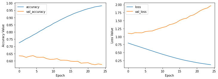
Using relu activation function got us to 25% accuracy so we changed it to softmax, and it easily helped us to get much higer accuracy as we can see above. So using softmax activation function in mid and last layer gave us high accuracy but after some iterations we could see that the model got overfitted and the best results happend in iterations 1 and 2!
Part b#
Use VGG16 network and report classification accuracy.
model_VGG16 = keras.applications.vgg16.VGG16(
    include_top=False,
    weights="imagenet",
    input_shape=(32, 32, 3),
#     pooling=None,
    classes=1000,
    classifier_activation="softmax",
)
1563/1563 [==============================] - 12s 8ms/step
model_VGG16.summary()
Model: "vgg16"
_________________________________________________________________
 Layer (type)                Output Shape              Param #
=================================================================
 input_2 (InputLayer)        [(None, 32, 32, 3)]       0

 block1_conv1 (Conv2D)       (None, 32, 32, 64)        1792

 block1_conv2 (Conv2D)       (None, 32, 32, 64)        36928

 block1_pool (MaxPooling2D)  (None, 16, 16, 64)        0

 block2_conv1 (Conv2D)       (None, 16, 16, 128)       73856

 block2_conv2 (Conv2D)       (None, 16, 16, 128)       147584

 block2_pool (MaxPooling2D)  (None, 8, 8, 128)         0

 block3_conv1 (Conv2D)       (None, 8, 8, 256)         295168

 block3_conv2 (Conv2D)       (None, 8, 8, 256)         590080

 block3_conv3 (Conv2D)       (None, 8, 8, 256)         590080

 block3_pool (MaxPooling2D)  (None, 4, 4, 256)         0

 block4_conv1 (Conv2D)       (None, 4, 4, 512)         1180160

 block4_conv2 (Conv2D)       (None, 4, 4, 512)         2359808

 block4_conv3 (Conv2D)       (None, 4, 4, 512)         2359808

 block4_pool (MaxPooling2D)  (None, 2, 2, 512)         0

 block5_conv1 (Conv2D)       (None, 2, 2, 512)         2359808

 block5_conv2 (Conv2D)       (None, 2, 2, 512)         2359808

 block5_conv3 (Conv2D)       (None, 2, 2, 512)         2359808

 block5_pool (MaxPooling2D)  (None, 1, 1, 512)         0

=================================================================
Total params: 14,714,688
Trainable params: 14,714,688
Non-trainable params: 0
_________________________________________________________________
y_pred_cifar = model_VGG16.predict(x_train_cifar)
y_pred_reshaped = np.reshape(y_pred_cifar, (50000, 512))
np.unique(np.argmax(y_pred_reshaped, axis=1))
array([155], dtype=int64)
the model predicted the class 155 only, and by this we can say that it is not working well, So we will use another method named transfer learning.
In transfer learning method, the learned concepts by a model will transfered to another model. Using the pre-trained model VGG16 we can create some layers on top of it and transfer the learned concept in the new layers.
base_model = keras.applications.vgg16.VGG16(weights='imagenet',
                                            include_top=False,
                                            input_shape=(32,32, 3))
base_model.trainable = False

model_vgg_transfer_learning = keras.models.Sequential([
    base_model,
    keras.layers.Flatten(),
    keras.layers.Dense(64, activation='relu'),
    keras.layers.Dense(32, activation='softmax'),
    keras.layers.Dense(10, activation='softmax')
])

model_vgg_transfer_learning.summary()
Model: "sequential_2"
_________________________________________________________________
 Layer (type)                Output Shape              Param #
=================================================================
 vgg16 (Functional)          (None, 1, 1, 512)         14714688

 flatten_2 (Flatten)         (None, 512)               0

 dense_4 (Dense)             (None, 64)                32832

 dense_5 (Dense)             (None, 32)                2080

 dense_6 (Dense)             (None, 10)                330

=================================================================
Total params: 14,749,930
Trainable params: 35,242
Non-trainable params: 14,714,688
_________________________________________________________________
model_vgg_transfer_learning.compile(optimizer='adam',
                                    loss=['categorical_crossentropy'],
                                    metrics=['accuracy'])

history_transfer_learning = model_vgg_transfer_learning.fit(x_train_cifar,
                                y_train_categorical_cifar,
                                batch_size=32, validation_split=0.1,
                                epochs=25)
Epoch 1/25
1407/1407 [==============================] - 21s 15ms/step - loss: 1.0895 - accuracy: 0.6239 - val_loss: 1.2294 - val_accuracy: 0.5756
Epoch 2/25
1407/1407 [==============================] - 18s 13ms/step - loss: 1.0702 - accuracy: 0.6337 - val_loss: 1.2038 - val_accuracy: 0.5870
Epoch 3/25
1407/1407 [==============================] - 19s 13ms/step - loss: 1.0529 - accuracy: 0.6389 - val_loss: 1.2131 - val_accuracy: 0.5892
Epoch 4/25
1407/1407 [==============================] - 19s 14ms/step - loss: 1.0405 - accuracy: 0.6452 - val_loss: 1.2015 - val_accuracy: 0.5848
Epoch 5/25
1407/1407 [==============================] - 19s 14ms/step - loss: 1.0239 - accuracy: 0.6506 - val_loss: 1.2211 - val_accuracy: 0.5856
Epoch 6/25
1407/1407 [==============================] - 19s 14ms/step - loss: 1.0102 - accuracy: 0.6561 - val_loss: 1.2135 - val_accuracy: 0.5912
Epoch 7/25
1407/1407 [==============================] - 19s 14ms/step - loss: 0.9973 - accuracy: 0.6614 - val_loss: 1.2065 - val_accuracy: 0.5978
Epoch 8/25
1407/1407 [==============================] - 19s 14ms/step - loss: 0.9848 - accuracy: 0.6671 - val_loss: 1.2371 - val_accuracy: 0.5930
Epoch 9/25
1407/1407 [==============================] - 19s 14ms/step - loss: 0.9738 - accuracy: 0.6733 - val_loss: 1.2233 - val_accuracy: 0.5976
Epoch 10/25
1407/1407 [==============================] - 19s 14ms/step - loss: 0.9616 - accuracy: 0.6764 - val_loss: 1.2064 - val_accuracy: 0.6038
Epoch 11/25
1407/1407 [==============================] - 20s 14ms/step - loss: 0.9518 - accuracy: 0.6794 - val_loss: 1.2084 - val_accuracy: 0.6004
Epoch 12/25
1407/1407 [==============================] - 20s 14ms/step - loss: 0.9433 - accuracy: 0.6807 - val_loss: 1.2221 - val_accuracy: 0.5976
Epoch 13/25
1407/1407 [==============================] - 20s 14ms/step - loss: 0.9333 - accuracy: 0.6893 - val_loss: 1.2160 - val_accuracy: 0.5974
Epoch 14/25
1407/1407 [==============================] - 20s 14ms/step - loss: 0.9242 - accuracy: 0.6889 - val_loss: 1.2391 - val_accuracy: 0.5952
Epoch 15/25
1407/1407 [==============================] - 20s 14ms/step - loss: 0.9150 - accuracy: 0.6923 - val_loss: 1.2477 - val_accuracy: 0.5958
Epoch 16/25
1407/1407 [==============================] - 20s 15ms/step - loss: 0.9093 - accuracy: 0.6951 - val_loss: 1.2363 - val_accuracy: 0.5978
Epoch 17/25
1407/1407 [==============================] - 20s 14ms/step - loss: 0.8983 - accuracy: 0.6984 - val_loss: 1.2184 - val_accuracy: 0.6012
Epoch 18/25
1407/1407 [==============================] - 20s 14ms/step - loss: 0.8916 - accuracy: 0.7028 - val_loss: 1.2531 - val_accuracy: 0.5926
Epoch 19/25
1407/1407 [==============================] - 20s 14ms/step - loss: 0.8876 - accuracy: 0.7045 - val_loss: 1.2563 - val_accuracy: 0.5992
Epoch 20/25
1407/1407 [==============================] - 20s 14ms/step - loss: 0.8793 - accuracy: 0.7060 - val_loss: 1.2627 - val_accuracy: 0.5974
Epoch 21/25
1407/1407 [==============================] - 20s 14ms/step - loss: 0.8721 - accuracy: 0.7094 - val_loss: 1.2726 - val_accuracy: 0.5940
Epoch 22/25
1407/1407 [==============================] - 22s 16ms/step - loss: 0.8678 - accuracy: 0.7093 - val_loss: 1.2678 - val_accuracy: 0.5992
Epoch 23/25
1407/1407 [==============================] - 20s 14ms/step - loss: 0.8623 - accuracy: 0.7109 - val_loss: 1.2809 - val_accuracy: 0.5980
Epoch 24/25
1407/1407 [==============================] - 20s 14ms/step - loss: 0.8555 - accuracy: 0.7151 - val_loss: 1.2795 - val_accuracy: 0.5934
Epoch 25/25
1407/1407 [==============================] - 20s 14ms/step - loss: 0.8499 - accuracy: 0.7168 - val_loss: 1.2832 - val_accuracy: 0.5942
plot_history(history_transfer_learning)
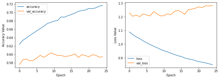
We again see that from the start the model tends to overfit because the accuracy is tending to go higher but for validation set the accuracy is not changing well and in loss is the same behaviour (training loss is decreasing but validation loss is increasing)
Fine tuning the model: To fine tune the transfer learning model we need to learn the pre-train model with a small learning rate and low count epochs.
base_model.trainable = True
model_vgg_transfer_learning.compile(
    optimizer=keras.optimizers.Adam(1e-5),
    loss=keras.losses.categorical_crossentropy,
    metrics=['accuracy']
)

history_transfer_learning_fine_tune = model_vgg_transfer_learning.fit(
    x_train_cifar,
    y_train_categorical_cifar,
    batch_size=32,
    validation_split=0.1,
    epochs=10
)
Epoch 1/10
1407/1407 [==============================] - 165s 116ms/step - loss: 0.9401 - accuracy: 0.6826 - val_loss: 0.9381 - val_accuracy: 0.6844
Epoch 2/10
1407/1407 [==============================] - 53s 38ms/step - loss: 0.7358 - accuracy: 0.7518 - val_loss: 0.7828 - val_accuracy: 0.7454
Epoch 3/10
1407/1407 [==============================] - 53s 38ms/step - loss: 0.6062 - accuracy: 0.7991 - val_loss: 0.7455 - val_accuracy: 0.7654
Epoch 4/10
1407/1407 [==============================] - 54s 38ms/step - loss: 0.5140 - accuracy: 0.8310 - val_loss: 0.7059 - val_accuracy: 0.7734
Epoch 5/10
1407/1407 [==============================] - 54s 38ms/step - loss: 0.4303 - accuracy: 0.8602 - val_loss: 0.6925 - val_accuracy: 0.7832
Epoch 6/10
1407/1407 [==============================] - 54s 39ms/step - loss: 0.3670 - accuracy: 0.8846 - val_loss: 0.6722 - val_accuracy: 0.7922
Epoch 7/10
1407/1407 [==============================] - 54s 38ms/step - loss: 0.3161 - accuracy: 0.9034 - val_loss: 0.6563 - val_accuracy: 0.7994
Epoch 8/10
1407/1407 [==============================] - 54s 39ms/step - loss: 0.2674 - accuracy: 0.9214 - val_loss: 0.6968 - val_accuracy: 0.7930
Epoch 9/10
1407/1407 [==============================] - 55s 39ms/step - loss: 0.2356 - accuracy: 0.9334 - val_loss: 0.6980 - val_accuracy: 0.7972
Epoch 10/10
1407/1407 [==============================] - 55s 39ms/step - loss: 0.2096 - accuracy: 0.9425 - val_loss: 0.6740 - val_accuracy: 0.8016
plot_history(history_transfer_learning_fine_tune)
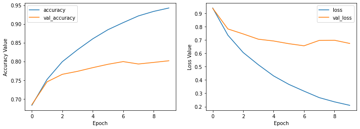
In the result of fine tuning we can see that exactly the performance of validation set with training set is increasing and this shows that the overfit effect here is vanished. Let’s see how this works with the test set.
test_loss, test_acc = model_vgg_transfer_learning.evaluate(x_test_cifar, y_test_cifar_categorical_cifar)
print(f'test accuracy: {test_acc}, test loss: {test_loss}')
313/313 [==============================] - 3s 11ms/step - loss: 0.7162 - accuracy: 0.7908
test accuracy: 0.7907999753952026, test loss: 0.7161977291107178
And finally our model is working well, let’s save it to be able to use it after re-running everything.
model_vgg_transfer_learning.save('Cifar_transfer_learning_model.h5')