HomeWork #1 Machine Learning#

Stu. name: Seyed Mohammad Amin Dadgar
Stu. no: 4003624016

import numpy as np
import pandas as pd
import seaborn as sns
import matplotlib.pyplot as plt
%matplotlib inline
import warnings
import scipy

Q2#

## column names are used from ```pima-indians-diabetes.name``` file
cols = ['pregnancy_count', 'glucose_test', 'blood_pressure', 'triceps_thickness', '2h_insulin', 'mass', 'pedi', 'age', 'label']

df = pd.read_csv('hw1_data/pima/pima-indians-diabetes.data', index_col=False ,names=cols)
df.head()

	pregnancy_count	glucose_test	blood_pressure	triceps_thickness	2h_insulin	mass	pedi	age	label
0	6	148	72	35	0	33.6	0.627	50	1
1	1	85	66	29	0	26.6	0.351	31	0
2	8	183	64	0	0	23.3	0.672	32	1
3	1	89	66	23	94	28.1	0.167	21	0
4	0	137	40	35	168	43.1	2.288	33	1

## save the dataset in the right format with its columns for other usages 
df.to_csv('hw1_data/processed/pima-indians-diabetes.csv')

(a, b)#

df.describe()

	pregnancy_count	glucose_test	blood_pressure	triceps_thickness	2h_insulin	mass	pedi	age	label
count	768.000000	768.000000	768.000000	768.000000	768.000000	768.000000	768.000000	768.000000	768.000000
mean	3.845052	120.894531	69.105469	20.536458	79.799479	31.992578	0.471876	33.240885	0.348958
std	3.369578	31.972618	19.355807	15.952218	115.244002	7.884160	0.331329	11.760232	0.476951
min	0.000000	0.000000	0.000000	0.000000	0.000000	0.000000	0.078000	21.000000	0.000000
25%	1.000000	99.000000	62.000000	0.000000	0.000000	27.300000	0.243750	24.000000	0.000000
50%	3.000000	117.000000	72.000000	23.000000	30.500000	32.000000	0.372500	29.000000	0.000000
75%	6.000000	140.250000	80.000000	32.000000	127.250000	36.600000	0.626250	41.000000	1.000000
max	17.000000	199.000000	122.000000	99.000000	846.000000	67.100000	2.420000	81.000000	1.000000

## the variance of each attribute
pd.DataFrame(df.var(), columns=['variance'])

	variance
pregnancy_count	11.354056
glucose_test	1022.248314
blood_pressure	374.647271
triceps_thickness	254.473245
2h_insulin	13281.180078
mass	62.159984
pedi	0.109779
age	138.303046
label	0.227483

(c)#

## Calculating the correlation between 8 attributes (label is outcluded)
attr_corr = df[cols[:-1]].corr()
attr_corr

	pregnancy_count	glucose_test	blood_pressure	triceps_thickness	2h_insulin	mass	pedi	age
pregnancy_count	1.000000	0.129459	0.141282	-0.081672	-0.073535	0.017683	-0.033523	0.544341
glucose_test	0.129459	1.000000	0.152590	0.057328	0.331357	0.221071	0.137337	0.263514
blood_pressure	0.141282	0.152590	1.000000	0.207371	0.088933	0.281805	0.041265	0.239528
triceps_thickness	-0.081672	0.057328	0.207371	1.000000	0.436783	0.392573	0.183928	-0.113970
2h_insulin	-0.073535	0.331357	0.088933	0.436783	1.000000	0.197859	0.185071	-0.042163
mass	0.017683	0.221071	0.281805	0.392573	0.197859	1.000000	0.140647	0.036242
pedi	-0.033523	0.137337	0.041265	0.183928	0.185071	0.140647	1.000000	0.033561
age	0.544341	0.263514	0.239528	-0.113970	-0.042163	0.036242	0.033561	1.000000

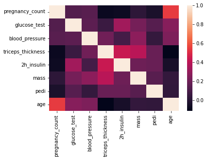
## showing the heatmap for better visualization
sns.heatmap(attr_corr)
plt.show()

label_corr = df.corrwith(df.label).sort_values(ascending=False)
pd.DataFrame(label_corr, columns=['correlation'])

	correlation
label	1.000000
glucose_test	0.466581
mass	0.292695
age	0.238356
pregnancy_count	0.221898
pedi	0.173844
2h_insulin	0.130548
triceps_thickness	0.074752
blood_pressure	0.065068

What we will find out from the correlation matrix with label is the most useful feature (Or the most affective feature ) for the label is glucose_test. To find why it is the most helpful attribute we can review the correlation formula with below \begin{equation} correlation = \frac{covariance(x,y)}{var(x) var(y)} \end{equation} And with this equation it’s obvious that if coefficient is positive then the effect of can be if x increases then y is increased. By this reason the biggest value for correlation of a feature with lable can be intrepreted the most helpful feature (attribute).

Also to explain the correlation value of one we can say that, x variable is the same as y in eq(1).

(d)#

If 2 attributes are fully correlated then using both in prediction may make bias and the prediction result would not be helpful. The alternative and the better way for prediction is to use one of the attributes.

(f)#

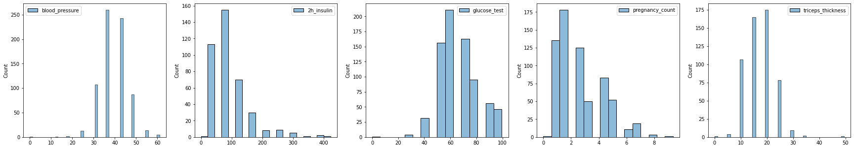
fig, ax = plt.subplots(3, 3, figsize=(15,9))
fig.tight_layout(pad=5)


sns.distplot(df.glucose_test, bins=20, ax=ax[0,0])
ax[0,0].set_title('Plasma glucose concentration a 2 hours\n in an oral glucose tolerance test')

sns.distplot(df.mass, bins=20, ax=ax[0,1])
ax[0, 1].set_title('Body mass index \n(weight in kg/(height in m)^2)')

sns.distplot(df.age, bins=20, ax=ax[0,2])
ax[0, 2].set_title('Age')

sns.distplot(df.pregnancy_count, bins=20, ax=ax[1,0])
ax[1, 0].set_title('Number of times pregnant')

sns.distplot(df.pedi, bins=20, ax=ax[1, 1])
ax[1, 1].set_title('Diabetes pedigree function')

sns.distplot(df['2h_insulin'], bins=20, ax=ax[1, 2])
ax[1, 2].set_title('2-Hour serum insulin (mu U/ml)')

sns.distplot(df.triceps_thickness, bins=20, ax=ax[2, 0])
ax[2, 0].set_title('Triceps skin fold thickness (mm)')

sns.distplot(df.blood_pressure, bins=20, ax=ax[2, 1])
ax[2, 1].set_title('Diastolic blood pressure (mm Hg)')

sns.distplot(df.label, bins=20, ax=ax[2, 2])
ax[2, 1].set_title('Class variable (0 or 1)')

plt.show()

/home/amin/.local/lib/python3.8/site-packages/seaborn/distributions.py:2619: FutureWarning: `distplot` is a deprecated function and will be removed in a future version. Please adapt your code to use either `displot` (a figure-level function with similar flexibility) or `histplot` (an axes-level function for histograms).
  warnings.warn(msg, FutureWarning)
/home/amin/.local/lib/python3.8/site-packages/seaborn/distributions.py:2619: FutureWarning: `distplot` is a deprecated function and will be removed in a future version. Please adapt your code to use either `displot` (a figure-level function with similar flexibility) or `histplot` (an axes-level function for histograms).
  warnings.warn(msg, FutureWarning)
/home/amin/.local/lib/python3.8/site-packages/seaborn/distributions.py:2619: FutureWarning: `distplot` is a deprecated function and will be removed in a future version. Please adapt your code to use either `displot` (a figure-level function with similar flexibility) or `histplot` (an axes-level function for histograms).
  warnings.warn(msg, FutureWarning)
/home/amin/.local/lib/python3.8/site-packages/seaborn/distributions.py:2619: FutureWarning: `distplot` is a deprecated function and will be removed in a future version. Please adapt your code to use either `displot` (a figure-level function with similar flexibility) or `histplot` (an axes-level function for histograms).
  warnings.warn(msg, FutureWarning)
/home/amin/.local/lib/python3.8/site-packages/seaborn/distributions.py:2619: FutureWarning: `distplot` is a deprecated function and will be removed in a future version. Please adapt your code to use either `displot` (a figure-level function with similar flexibility) or `histplot` (an axes-level function for histograms).
  warnings.warn(msg, FutureWarning)
/home/amin/.local/lib/python3.8/site-packages/seaborn/distributions.py:2619: FutureWarning: `distplot` is a deprecated function and will be removed in a future version. Please adapt your code to use either `displot` (a figure-level function with similar flexibility) or `histplot` (an axes-level function for histograms).
  warnings.warn(msg, FutureWarning)
/home/amin/.local/lib/python3.8/site-packages/seaborn/distributions.py:2619: FutureWarning: `distplot` is a deprecated function and will be removed in a future version. Please adapt your code to use either `displot` (a figure-level function with similar flexibility) or `histplot` (an axes-level function for histograms).
  warnings.warn(msg, FutureWarning)
/home/amin/.local/lib/python3.8/site-packages/seaborn/distributions.py:2619: FutureWarning: `distplot` is a deprecated function and will be removed in a future version. Please adapt your code to use either `displot` (a figure-level function with similar flexibility) or `histplot` (an axes-level function for histograms).
  warnings.warn(msg, FutureWarning)
/home/amin/.local/lib/python3.8/site-packages/seaborn/distributions.py:2619: FutureWarning: `distplot` is a deprecated function and will be removed in a future version. Please adapt your code to use either `displot` (a figure-level function with similar flexibility) or `histplot` (an axes-level function for histograms).
  warnings.warn(msg, FutureWarning)

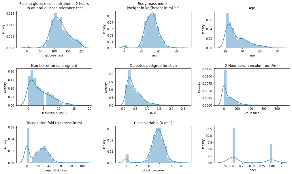
If we look closely we can say that body mass index and the plasma glucose is the most similar to normal distribution.

fig, ax = plt.subplots(3, 3, figsize=(20,15))
fig.tight_layout(pad=5)



sns.scatterplot(df.glucose_test,df.mass, ax=ax[0,0])
ax[0,0].legend(['glucose_test And mass'])

sns.scatterplot(df.mass, df.age, ax=ax[0,1])
ax[0, 1].legend(['mass And age'])


sns.scatterplot(df.age, df.pregnancy_count, ax=ax[0,2])
ax[0, 2].legend(['age And pregnancy_count'])

sns.scatterplot(df.pregnancy_count, df.pedi, ax=ax[1,0])
ax[1, 0].legend(['pregnancy_count And predi'])

sns.scatterplot(df.pedi, df['2h_insulin'], ax=ax[1, 1])
ax[1, 1].legend(['predi And 2h_insulin'])

sns.scatterplot(df['2h_insulin'], df.triceps_thickness, ax=ax[1, 2])
ax[1, 2].legend(['2h_insulin And triceps_thickness'])

sns.scatterplot(df.triceps_thickness, df.blood_pressure, ax=ax[2, 0])
ax[2, 0].legend(['triceps_thickness And blood_pressure'])

ax[2,1].set_axis_off()
ax[2,2].set_axis_off()

plt.show()

/home/amin/.local/lib/python3.8/site-packages/seaborn/_decorators.py:36: FutureWarning: Pass the following variables as keyword args: x, y. From version 0.12, the only valid positional argument will be `data`, and passing other arguments without an explicit keyword will result in an error or misinterpretation.
  warnings.warn(
/home/amin/.local/lib/python3.8/site-packages/seaborn/_decorators.py:36: FutureWarning: Pass the following variables as keyword args: x, y. From version 0.12, the only valid positional argument will be `data`, and passing other arguments without an explicit keyword will result in an error or misinterpretation.
  warnings.warn(
/home/amin/.local/lib/python3.8/site-packages/seaborn/_decorators.py:36: FutureWarning: Pass the following variables as keyword args: x, y. From version 0.12, the only valid positional argument will be `data`, and passing other arguments without an explicit keyword will result in an error or misinterpretation.
  warnings.warn(
/home/amin/.local/lib/python3.8/site-packages/seaborn/_decorators.py:36: FutureWarning: Pass the following variables as keyword args: x, y. From version 0.12, the only valid positional argument will be `data`, and passing other arguments without an explicit keyword will result in an error or misinterpretation.
  warnings.warn(
/home/amin/.local/lib/python3.8/site-packages/seaborn/_decorators.py:36: FutureWarning: Pass the following variables as keyword args: x, y. From version 0.12, the only valid positional argument will be `data`, and passing other arguments without an explicit keyword will result in an error or misinterpretation.
  warnings.warn(
/home/amin/.local/lib/python3.8/site-packages/seaborn/_decorators.py:36: FutureWarning: Pass the following variables as keyword args: x, y. From version 0.12, the only valid positional argument will be `data`, and passing other arguments without an explicit keyword will result in an error or misinterpretation.
  warnings.warn(
/home/amin/.local/lib/python3.8/site-packages/seaborn/_decorators.py:36: FutureWarning: Pass the following variables as keyword args: x, y. From version 0.12, the only valid positional argument will be `data`, and passing other arguments without an explicit keyword will result in an error or misinterpretation.
  warnings.warn(

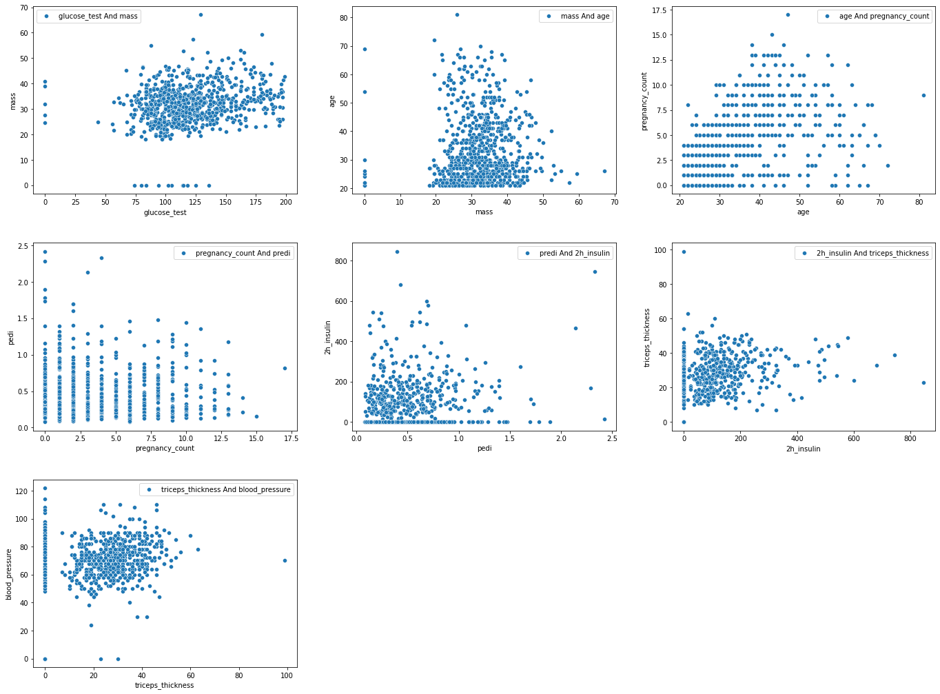
It is obvious that for (pregnancy_count, predi) and (age, pregnancy_count) we can say they have linear dependency.

Q3#

(a)#

create a normalize function using the equation below \begin{equation} x_{norm} = \frac{x- \mu_x}{\sigma_x} \end{equation} normalize the third attribute on pima dataset, then report the values for the first 5 entries on dataset.

## column names are used from ```pima-indians-diabetes.name``` file
cols = ['pregnancy_count', 'glucose_test', 'blood_pressure', 'triceps_thickness', '2h_insulin', 'mass', 'pedi', 'age', 'label']

df = pd.read_csv('hw1_data/pima/pima-indians-diabetes.data', index_col=False ,names=cols)
df.head()

	pregnancy_count	glucose_test	blood_pressure	triceps_thickness	2h_insulin	mass	pedi	age	label
0	6	148	72	35	0	33.6	0.627	50	1
1	1	85	66	29	0	26.6	0.351	31	0
2	8	183	64	0	0	23.3	0.672	32	1
3	1	89	66	23	94	28.1	0.167	21	0
4	0	137	40	35	168	43.1	2.288	33	1

def normalize(attrib):
    """
    normalize an attribute using its mean and standard deviation

    INPUTS:
    --------
    attrib: a pandas series, the original unormalized attribute

    OUTPUT:
    --------
    normalized:  the normalized attribute
    """

    mu = attrib.mean()
    sigma = attrib.std()

    normalized = (attrib - mu) / sigma
    return normalized

## third attribute is blood pressure
blood_pressure_norm = normalize(df.blood_pressure)
pd.DataFrame(blood_pressure_norm)

	blood_pressure
0	0.149543
1	-0.160441
2	-0.263769
3	-0.160441
4	-1.503707
...	...
763	0.356200
764	0.046215
765	0.149543
766	-0.470426
767	0.046215

768 rows × 1 columns

## normalize first 5 attribute of the function
normalize(df[['pregnancy_count', 'glucose_test', 'blood_pressure', 'triceps_thickness', '2h_insulin']])

	pregnancy_count	glucose_test	blood_pressure	triceps_thickness	2h_insulin
0	0.639530	0.847771	0.149543	0.906679	-0.692439
1	-0.844335	-1.122665	-0.160441	0.530556	-0.692439
2	1.233077	1.942458	-0.263769	-1.287373	-0.692439
3	-0.844335	-0.997558	-0.160441	0.154433	0.123221
4	-1.141108	0.503727	-1.503707	0.906679	0.765337
...	...	...	...	...	...
763	1.826623	-0.622237	0.356200	1.721613	0.869464
764	-0.547562	0.034575	0.046215	0.405181	-0.692439
765	0.342757	0.003299	0.149543	0.154433	0.279412
766	-0.844335	0.159683	-0.470426	-1.287373	-0.692439
767	-0.844335	-0.872451	0.046215	0.655930	-0.692439

768 rows × 5 columns

new_df = df[['pregnancy_count', 'glucose_test', 'triceps_thickness', '2h_insulin']].copy()
new_df['normalized_blood_pressure'] = blood_pressure_norm
new_df.head()

	pregnancy_count	glucose_test	triceps_thickness	2h_insulin	normalized_blood_pressure
0	6	148	35	0	0.149543
1	1	85	29	0	-0.160441
2	8	183	0	0	-0.263769
3	1	89	23	94	-0.160441
4	0	137	35	168	-1.503707

(b)#

def discretize_attribute(attribute ,bins=10, verbose=False):
    """
    descritize a continues attribute and make the intervals the bins size

    INPUTS:
    --------
    attribute: pandas series of **one column**
    bins:  the interval space for each class, default is 10
    verbose: print the each stage output if True, default is False

    OUTPUT:
    --------
    pandas dataframe of the discrite values of an attribute 
    """
    list = np.empty((1,len(attribute.columns)))

    ## each bin length 
    bin_len = attribute.max().max() / bins
    # bin_len = int(bin_len)

    if verbose: print(f'bin length: {bin_len}')
    
    ## counter to iterate the intervals
    interval = 0
    while interval < attribute.max().max():
        ## find the attributes within the interval and drop na (NAN values are thoes who are not in the interval)
        conditioned_data = attribute.where((interval < attribute) & (attribute < interval + bin_len)).dropna().values
        
        if verbose: print(conditioned_data)
        
        ## To discretize the attributes set all the values to the mean of interval we have
        conditioned_data[True] = (interval + bin_len) / 2

        list = np.append(list, conditioned_data, axis=0 )
        ## iterate the next intervals
        interval += bin_len


    return pd.DataFrame(list, columns=attribute.columns, dtype='float32')
    

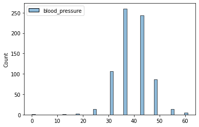
attrib = df[['blood_pressure']]
df_discrete_blood_pressure =  discretize_attribute(attrib, 10)
df_discrete_blood_pressure

	blood_pressure
0	0.000000
1	12.200000
2	18.299999
3	18.299999
4	24.400000
...	...
728	61.000000
729	61.000000
730	61.000000
731	61.000000
732	61.000000

733 rows × 1 columns

sns.histplot(df_discrete_blood_pressure)
plt.show()

df_discrete_pregnancy = discretize_attribute(df[['pregnancy_count']], 10)
df_discrete_glucose_test = discretize_attribute(df[['glucose_test']], 10)
df_discrete_triceps_thickness = discretize_attribute(df[['triceps_thickness']], 10)
df_discrete_2h_insulin = discretize_attribute(df[['2h_insulin']], 10)

fig, axes = plt.subplots(1, 5, figsize=(30, 5))
sns.histplot(df_discrete_blood_pressure, ax=axes[0])
sns.histplot(df_discrete_2h_insulin, ax=axes[1])
sns.histplot(df_discrete_glucose_test, ax=axes[2])
sns.histplot(df_discrete_pregnancy, ax=axes[3])
sns.histplot(df_discrete_triceps_thickness, ax=axes[4])

plt.show()

Q4#

(a)#

## column names are used from ```pima-indians-diabetes.name``` file
cols = ['pregnancy_count', 'glucose_test', 'blood_pressure', 'triceps_thickness', '2h_insulin', 'mass', 'pedi', 'age', 'label']

df = pd.read_csv('hw1_data/pima/pima-indians-diabetes.data', index_col=False ,names=cols)
df.head()

	pregnancy_count	glucose_test	blood_pressure	triceps_thickness	2h_insulin	mass	pedi	age	label
0	6	148	72	35	0	33.6	0.627	50	1
1	1	85	66	29	0	26.6	0.351	31	0
2	8	183	64	0	0	23.3	0.672	32	1
3	1	89	66	23	94	28.1	0.167	21	0
4	0	137	40	35	168	43.1	2.288	33	1

df_class_0 = df[df.label == 0].copy()
df_class_1 = df[df.label == 1].copy()

df_class_0.describe()

	pregnancy_count	glucose_test	blood_pressure	triceps_thickness	2h_insulin	mass	pedi	age	label
count	500.000000	500.0000	500.000000	500.000000	500.000000	500.000000	500.000000	500.000000	500.0
mean	3.298000	109.9800	68.184000	19.664000	68.792000	30.304200	0.429734	31.190000	0.0
std	3.017185	26.1412	18.063075	14.889947	98.865289	7.689855	0.299085	11.667655	0.0
min	0.000000	0.0000	0.000000	0.000000	0.000000	0.000000	0.078000	21.000000	0.0
25%	1.000000	93.0000	62.000000	0.000000	0.000000	25.400000	0.229750	23.000000	0.0
50%	2.000000	107.0000	70.000000	21.000000	39.000000	30.050000	0.336000	27.000000	0.0
75%	5.000000	125.0000	78.000000	31.000000	105.000000	35.300000	0.561750	37.000000	0.0
max	13.000000	197.0000	122.000000	60.000000	744.000000	57.300000	2.329000	81.000000	0.0

df_class_1.describe()

	pregnancy_count	glucose_test	blood_pressure	triceps_thickness	2h_insulin	mass	pedi	age	label
count	268.000000	268.000000	268.000000	268.000000	268.000000	268.000000	268.000000	268.000000	268.0
mean	4.865672	141.257463	70.824627	22.164179	100.335821	35.142537	0.550500	37.067164	1.0
std	3.741239	31.939622	21.491812	17.679711	138.689125	7.262967	0.372354	10.968254	0.0
min	0.000000	0.000000	0.000000	0.000000	0.000000	0.000000	0.088000	21.000000	1.0
25%	1.750000	119.000000	66.000000	0.000000	0.000000	30.800000	0.262500	28.000000	1.0
50%	4.000000	140.000000	74.000000	27.000000	0.000000	34.250000	0.449000	36.000000	1.0
75%	8.000000	167.000000	82.000000	36.000000	167.250000	38.775000	0.728000	44.000000	1.0
max	17.000000	199.000000	114.000000	99.000000	846.000000	67.100000	2.420000	70.000000	1.0

(b)#

## we would choose randomly an index with the probability of 66% 
def divideset1(df, prob=0.66):
    """
    divide the dataset into train and test with a probability

    INPUTS:
    --------
    df: pandas dataframe, the dataset we want to split
    prob: the probability to divide the dataset, default is 0.66

    OUTPUTS:
    ---------
    train: pandas dataframe, the portion of the dataset for train
    test: pandas dataframe, the portion of the dataset for test
    """
    ## copy the dataframe to ensure there is no problem
    dataset = df.copy()

    trainset = pd.DataFrame(columns=dataset.columns)
    testset = pd.DataFrame(columns=dataset.columns)

    ## iterate over dataset and select each row as train or test
    for i in range(0, len(dataset)):
        ## get the row
        row = dataset.iloc[0]

        probability = np.random.random()
        ## if the probability range is between 0 and chosen prob
        if probability - prob > 0:
            trainset = trainset.append(row)
        else:
            testset = testset.append(row)

    return trainset, testset

train_split, test_split = divideset1(df)
train_split

	pregnancy_count	glucose_test	blood_pressure	triceps_thickness	2h_insulin	mass	pedi	age	label
0	6.0	148.0	72.0	35.0	0.0	33.6	0.627	50.0	1.0
0	6.0	148.0	72.0	35.0	0.0	33.6	0.627	50.0	1.0
0	6.0	148.0	72.0	35.0	0.0	33.6	0.627	50.0	1.0
0	6.0	148.0	72.0	35.0	0.0	33.6	0.627	50.0	1.0
0	6.0	148.0	72.0	35.0	0.0	33.6	0.627	50.0	1.0
...	...	...	...	...	...	...	...	...	...
0	6.0	148.0	72.0	35.0	0.0	33.6	0.627	50.0	1.0
0	6.0	148.0	72.0	35.0	0.0	33.6	0.627	50.0	1.0
0	6.0	148.0	72.0	35.0	0.0	33.6	0.627	50.0	1.0
0	6.0	148.0	72.0	35.0	0.0	33.6	0.627	50.0	1.0
0	6.0	148.0	72.0	35.0	0.0	33.6	0.627	50.0	1.0

249 rows × 9 columns

## check the average training split size with the count of times
times = 20
## save all lengths
lengths = []
for i in range(times):
    training_len = len(divideset1(df)[0])
    print(f'Iteration {i} - training length: {training_len}')
    lengths.append(training_len)
print('------------------------------------------')
print(f'Average Lengths: {np.average(lengths)}')

Iteration 0 - training length: 255
Iteration 1 - training length: 256
Iteration 2 - training length: 273
Iteration 3 - training length: 250
Iteration 4 - training length: 244
Iteration 5 - training length: 237
Iteration 6 - training length: 250
Iteration 7 - training length: 247
Iteration 8 - training length: 257
Iteration 9 - training length: 259
Iteration 10 - training length: 240
Iteration 11 - training length: 238
Iteration 12 - training length: 270
Iteration 13 - training length: 267
Iteration 14 - training length: 248
Iteration 15 - training length: 248
Iteration 16 - training length: 273
Iteration 17 - training length: 257
Iteration 18 - training length: 259
Iteration 19 - training length: 247
------------------------------------------
Average Lengths: 253.75

(c)#

def divideset2(df, fraction = 0.66):
    """
    Divide the dataset into train and test with fixed size every run

    INPUTS:
    ---------
    df: pandas dataframe, the dataset that is going to be splitted
    fraction: the value to divide the dataset, default is 0.66

    OUTPUTS:
    ---------
    train: pandas dataframe, the portion of the dataset for train
    test: pandas dataframe, the portion of the dataset for test
    """

    train = df.sample(frac=0.66).copy()
    test = df.drop(train.index)

    return train, test

train2, test2 = divideset2(df)

print(train2.head())
print('-----------------------'* 10)
print(test2.head())

     pregnancy_count  glucose_test  blood_pressure  triceps_thickness  \
              7           114              64                  0   
              0           100              70                 26   
              8           120               0                  0   
              2           175              88                  0   
              1           109              60                  8   

     2h_insulin  mass   pedi  age  label  
         0  27.4  0.732   34      1  
        50  30.8  0.597   21      0  
         0  30.0  0.183   38      1  
         0  22.9  0.326   22      0  
       182  25.4  0.947   21      0  
--------------------------------------------------------------------------------------------------------------------------------------------------------------------------------------------------------------------------------------
    pregnancy_count  glucose_test  blood_pressure  triceps_thickness  \
               6           148              72                 35   
               8           183              64                  0   
               1            89              66                 23   
               3            78              50                 32   
             10           168              74                  0   

    2h_insulin  mass   pedi  age  label  
          0  33.6  0.627   50      1  
          0  23.3  0.672   32      1  
         94  28.1  0.167   21      0  
         88  31.0  0.248   26      1  
         0  38.0  0.537   34      1  

Validation schemes#

(a) K-fold Cross Validation#

def kfold_crossvalidation(data, k, m):
    """
    K-fold cross validation 
    Note: test data is equivalent the validation data in normal machine learning models (Because it is used to evaluate one model)

    INPUTS:
    --------
    data: pandas dataframe containing feature vectors as rows
    k: positive integer, the number of folds
    m: target output 
    train_split:  the fraction of data that is used to split for training, default is 0.7

    OUTPUTS:
    ---------
    training_data: multi-dimensional array of training data, each index contains the dataset for K-fold number
    test_data: multi-dimensional array of test data, each ```index+1``` contains the dataset for each K-fold number
    """
    ## get the length of data to split it
    dataframe_size = len(data)

    ## find the length of each split
    # training_size = int(dataframe_size * train_split)
    # test_size = dataframe_size - training_size

    ## empty arrays to save data into it
    training_data = []
    test_data = []

    ## find the split size
    split = int(dataframe_size / k)

    ## split the data into k-fold and add the folds into the arrays
    for i in range(k):
        start_idx = int(i*split)
        end_idx = int((i+1)*split)

        test = data.iloc[start_idx:end_idx].copy()
        ## add the label column to corresponding index
        test['label'] = m.iloc[start_idx: end_idx]
        
        
        ## choose other part of dataset as train
        train = pd.concat([data, test, test]).drop_duplicates(keep=False)
        train['label'] = m.iloc[train.index]
        
        training_data.append(train)
        test_data.append(test)

    return training_data, test_data

K = 5
training_folds, test_folds = kfold_crossvalidation(df, K, df.label )

## check the K=1 test data fold
test_folds[0]

	pregnancy_count	glucose_test	blood_pressure	triceps_thickness	2h_insulin	mass	pedi	age	label
0	6	148	72	35	0	33.6	0.627	50	1
1	1	85	66	29	0	26.6	0.351	31	0
2	8	183	64	0	0	23.3	0.672	32	1
3	1	89	66	23	94	28.1	0.167	21	0
4	0	137	40	35	168	43.1	2.288	33	1
...	...	...	...	...	...	...	...	...	...
148	5	147	78	0	0	33.7	0.218	65	0
149	2	90	70	17	0	27.3	0.085	22	0
150	1	136	74	50	204	37.4	0.399	24	0
151	4	114	65	0	0	21.9	0.432	37	0
152	9	156	86	28	155	34.3	1.189	42	1

153 rows × 9 columns

## check K=1 fold training set 
training_folds[0]

	pregnancy_count	glucose_test	blood_pressure	triceps_thickness	2h_insulin	mass	pedi	age	label
153	1	153	82	42	485	40.6	0.687	23	0
154	8	188	78	0	0	47.9	0.137	43	1
155	7	152	88	44	0	50.0	0.337	36	1
156	2	99	52	15	94	24.6	0.637	21	0
157	1	109	56	21	135	25.2	0.833	23	0
...	...	...	...	...	...	...	...	...	...
763	10	101	76	48	180	32.9	0.171	63	0
764	2	122	70	27	0	36.8	0.340	27	0
765	5	121	72	23	112	26.2	0.245	30	0
766	1	126	60	0	0	30.1	0.349	47	1
767	1	93	70	31	0	30.4	0.315	23	0

615 rows × 9 columns

## we can see that the test and train summation size matches the whole dataframe
for k in range(K):
    ## does it maches the whole dataset size? (condition variable)
    condition = (len(df) == (len(training_folds[k]) + len(test_folds[k]))) 
    print(f'Fold K={k+1}, the summation matches the whole set, {condition}')

Fold K=1, the summation matches the whole set, True
Fold K=2, the summation matches the whole set, True
Fold K=3, the summation matches the whole set, True
Fold K=4, the summation matches the whole set, True
Fold K=5, the summation matches the whole set, True

(b) Bootstraping#

def bootstrap1(data):
    """
    Demonstrate one iteration of bootstraping method (it is a with replacement method)

    INPUT:
    -------
    data: a pandas dataframe, containing our data

    OUPUTS:
    --------
    train_data: pandas dataframe of a sample data
    test_data: pandas dataframe of sample data, the data that are not included in train_data
    """
    ## find the length of our data (how many data rows we have)
    data_length = len(data)
    
    ## the indexes to be chosen from original data 
    indexes = np.random.randint(data_length, size=data_length)
    
    ## create the training set
    train_data = df.iloc[indexes].copy()

    ## choose the test set, (The data that is omited from training set)
    test_data = pd.concat([data,train_data, train_data]).drop_duplicates(keep=False)

    return train_data, test_data

bootstrap_train, bootstrap_test = bootstrap1(df)

## check the training set length with original data
len(bootstrap_train) == len(df)

True

print(len(bootstrap_train))
bootstrap_train.head()

	pregnancy_count	glucose_test	blood_pressure	triceps_thickness	2h_insulin	mass	pedi	age	label
455	14	175	62	30	0	33.6	0.212	38	1
67	2	109	92	0	0	42.7	0.845	54	0
692	2	121	70	32	95	39.1	0.886	23	0
191	9	123	70	44	94	33.1	0.374	40	0
711	5	126	78	27	22	29.6	0.439	40	0

print(len(bootstrap_test))
bootstrap_test.head()

	pregnancy_count	glucose_test	blood_pressure	triceps_thickness	2h_insulin	mass	pedi	age	label
1	1	85	66	29	0	26.6	0.351	31	0
3	1	89	66	23	94	28.1	0.167	21	0
8	2	197	70	45	543	30.5	0.158	53	1
12	10	139	80	0	0	27.1	1.441	57	0
16	0	118	84	47	230	45.8	0.551	31	1

Q7#

(f)#

def poisson_distribution(X,lambda1):
    """
    poisson distribution function

    INPUT:
    --------
    X: integer or an array of integers, the input value
    lambda1: float, hyperparameter to set 

    OUTPUT:
    ---------
    probabiltiy: type is same as input, the probability distribution of X
    """
    ## calculate the value above the division and below separately
    above_division = np.exp(- lambda1) * np.power(lambda1, X)
    under_division = scipy.special.factorial(X)

    
    return np.divide(above_division, under_division)

## parameter lambda = 2
X = np.linspace(0, 10, 50)
Y1 = poisson_distribution(X, lambda1=2)
plt.plot(X, Y1)
plt.show()

## parameter lambda = 6
X = np.linspace(0, 10, 50)
Y1 = poisson_distribution(X, lambda1=6)
plt.plot(X, Y1)
plt.show()

(g)#

The Maximum Likelihood estimation for poisson distribution is as below (Calculated in Q7 part c) \begin{equation} \lambda = \frac{1}{n} \sum_{i=0}^{n} x_i \end{equation}

## Read the data from poisson.txt file
X_poisson = np.fromfile('hw1_data/poisson.txt', dtype=float, sep='\n')
## Maximum Likelihood estimation
lambda1 = np.sum(X_poisson) / len(X_poisson)

print('Maximum Likelihood Estimated Parameter for poisson.txt: ', lambda1)

Maximum Likelihood Estimated Parameter for poisson.txt:  5.24

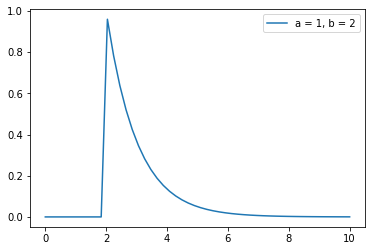
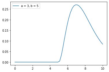
(h)#

X = np.linspace(0, 10, 50)
gamma_model = scipy.stats.gamma(1,2)
plt.plot(X, gamma_model.pdf(X))
plt.legend(['a = 1, b = 2'])
plt.show()

X = np.linspace(0, 10, 50)
gamma_model = scipy.stats.gamma(3,5)
plt.plot(X, gamma_model.pdf(X))
plt.legend(['a = 3, b = 5'])
plt.show()

(i)#

Posterior density can be found as \begin{equation} Posterior = Likelihood \times Prior \end{equation} The prior of probability is \begin{equation} P(x) = \frac{e^{-\lambda} \lambda^x}{x!} \end{equation} \begin{equation} p(\lambda | a,b) = \frac{1}{b^a \Gamma(a)} \lambda^{a-1} e^{-\frac{\lambda}{b}} \end{equation} And assuming the poisson.txt file we found the proper value for lambda

def posterior_poisson(X, a,b, lambda1):
    """
    posterior for poisson distribution

    INPUTS:
    -------
    X: values to calculate the posterior
    a,b: parameters for gamma distribution

    OUTPUT:
    --------
    probability: floating number or an array
    """
    ## we divided the function in 3 parts then multiplied it
    gamma_distro = scipy.stats.gamma(a)
    values = gamma_distro.pdf(X)
    p1 = (b ** a) * values
    p1 = 1 / p1

    p2 = lambda1 ** (a-1)
    
    p3 = np.exp(-lambda1 / b)

    probability = p1 * p2 * p3
    print(len(probability))
    return probability

Y = posterior_poisson(X_poisson, 3, 5, lambda1)
plt.figure(figsize=(8,6))
plt.plot(X_poisson,Y)
plt.legend(['Posterior distribution with a=1, b=2'])
plt.show()

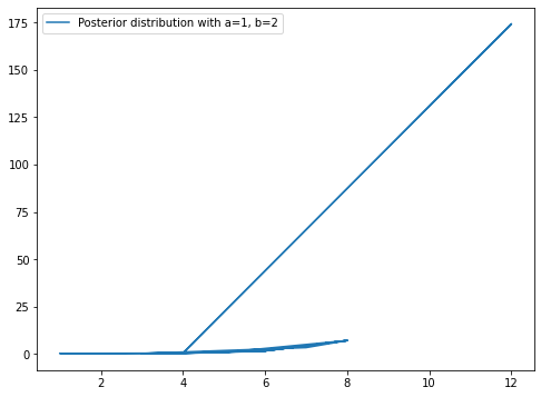
It can be seen from the plot that the posterior is not a function and it have multiple values of x for each y in range of 4 to 8.

Q8#

Part 1#

(a)#

## read the data from housing.txt
## there is one or more space for each data
columns = ['CRIM', 'ZN', 'INDUS', 'CHAS', 'NOX', 'RM', 'AGE', 'DIS', 'RAD','TAX', 'PTRATIO', 'B', 'LSTAT', 'MEDV']
df_boston = pd.read_csv('hw1_data/housing/housing.txt', sep= ' +', index_col=False, names=columns)

/home/amin/.local/lib/python3.8/site-packages/pandas/util/_decorators.py:311: ParserWarning: Falling back to the 'python' engine because the 'c' engine does not support regex separators (separators > 1 char and different from '\s+' are interpreted as regex); you can avoid this warning by specifying engine='python'.
  return func(*args, **kwargs)

df_boston.head()

	CRIM	ZN	INDUS	NOX	RM	AGE	DIS	RAD	TAX	PTRATIO	B	LSTAT	MEDV
0	0.00632	18.0	2.31	0.538	6.575	65.2	4.0900	1	296.0	15.3	396.90	4.98	24.0
1	0.02731	0.0	7.07	0.469	6.421	78.9	4.9671	2	242.0	17.8	396.90	9.14	21.6
2	0.02729	0.0	7.07	0.469	7.185	61.1	4.9671	2	242.0	17.8	392.83	4.03	34.7
3	0.03237	0.0	2.18	0.458	6.998	45.8	6.0622	3	222.0	18.7	394.63	2.94	33.4
4	0.06905	0.0	2.18	0.458	7.147	54.2	6.0622	3	222.0	18.7	396.90	5.33	36.2

df_boston.dtypes

CRIM       float64
ZN         float64
INDUS      float64
CHAS         int64
NOX        float64
RM         float64
AGE        float64
DIS        float64
RAD          int64
TAX        float64
PTRATIO    float64
B          float64
LSTAT      float64
MEDV       float64
dtype: object

As we can see there is no attribute type as object, so we will look at the dataset closely.

df_boston.CHAS.value_counts()

0    471
1     35
Name: CHAS, dtype: int64

It is clear here that CHAS is a binary feature.

df_boston.ZN.value_counts()

0      372
0      21
0      15
0      10
5      10
0      10
0       7
0       6
0       6
0       5
0       4
0       4
0       4
0       4
0       3
0       3
0       3
5       3
0       3
0       3
0       3
5       2
0       2
5       1
0      1
0       1
Name: ZN, dtype: int64

So after having a look at dataset and two of the features we saw that just one of the columns have binary value, and it is the CHAS.

(b)#

correlation = df_boston[columns[:-1]].corrwith(df_boston.MEDV).sort_values(ascending=True)
pd.DataFrame(correlation, columns=['correlation with MEDV'])

	correlation with MEDV
LSTAT	-0.737663
PTRATIO	-0.507787
INDUS	-0.483725
TAX	-0.468536
NOX	-0.427321
CRIM	-0.388305
RAD	-0.381626
AGE	-0.376955
CHAS	0.175260
DIS	0.249929
B	0.333461
ZN	0.360445
RM	0.695360

It is clear from above that:
Highest Positive Correlation: RM
Highest Negative Correlation: LSTAT

(c)#

fig, axes = plt.subplots(3, 5, figsize=(25, 10))
fig.tight_layout(pad=5)

sns.scatterplot(x=df_boston.LSTAT, y=df_boston.MEDV, ax=axes[0,0])
sns.scatterplot(x=df_boston.PTRATIO, y=df_boston.MEDV, ax=axes[0,1])
sns.scatterplot(x=df_boston.INDUS, y=df_boston.MEDV, ax=axes[0,2])
sns.scatterplot(x=df_boston.TAX, y=df_boston.MEDV, ax=axes[0,3])
sns.scatterplot(x=df_boston.NOX, y=df_boston.MEDV, ax=axes[0,4])
sns.scatterplot(x=df_boston.CRIM, y=df_boston.MEDV, ax=axes[1,0])
sns.scatterplot(x=df_boston.AGE, y=df_boston.MEDV, ax=axes[1,1])
sns.scatterplot(x=df_boston.CHAS, y=df_boston.MEDV, ax=axes[1,2])
sns.scatterplot(x=df_boston.DIS, y=df_boston.MEDV, ax=axes[1,3])
sns.scatterplot(x=df_boston.B, y=df_boston.MEDV, ax=axes[1,4])
sns.scatterplot(x=df_boston.ZN, y=df_boston.MEDV, ax=axes[2,0])
sns.scatterplot(x=df_boston.RM, y=df_boston.MEDV, ax=axes[2,1])
axes[2,2].set_axis_off()
axes[2,3].set_axis_off()
axes[2,4].set_axis_off()

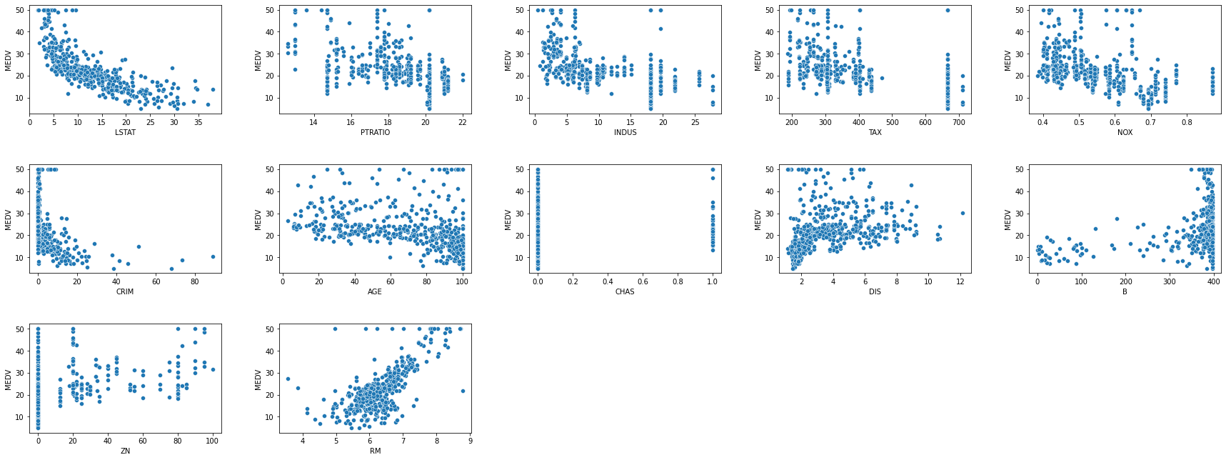
The most correlated features are having the most linear scatter plot. As we can see from the scatter plots, RM and LSTAT are in the most linear form.

(d)#

df_boston.corr()

	CRIM	ZN	INDUS	CHAS	NOX	RM	AGE	DIS	RAD	TAX	PTRATIO	B	LSTAT	MEDV
CRIM	1.000000	-0.200469	0.406583	-0.055892	0.420972	-0.219247	0.352734	-0.379670	0.625505	0.582764	0.289946	-0.385064	0.455621	-0.388305
ZN	-0.200469	1.000000	-0.533828	-0.042697	-0.516604	0.311991	-0.569537	0.664408	-0.311948	-0.314563	-0.391679	0.175520	-0.412995	0.360445
INDUS	0.406583	-0.533828	1.000000	0.062938	0.763651	-0.391676	0.644779	-0.708027	0.595129	0.720760	0.383248	-0.356977	0.603800	-0.483725
CHAS	-0.055892	-0.042697	0.062938	1.000000	0.091203	0.091251	0.086518	-0.099176	-0.007368	-0.035587	-0.121515	0.048788	-0.053929	0.175260
NOX	0.420972	-0.516604	0.763651	0.091203	1.000000	-0.302188	0.731470	-0.769230	0.611441	0.668023	0.188933	-0.380051	0.590879	-0.427321
RM	-0.219247	0.311991	-0.391676	0.091251	-0.302188	1.000000	-0.240265	0.205246	-0.209847	-0.292048	-0.355501	0.128069	-0.613808	0.695360
AGE	0.352734	-0.569537	0.644779	0.086518	0.731470	-0.240265	1.000000	-0.747881	0.456022	0.506456	0.261515	-0.273534	0.602339	-0.376955
DIS	-0.379670	0.664408	-0.708027	-0.099176	-0.769230	0.205246	-0.747881	1.000000	-0.494588	-0.534432	-0.232471	0.291512	-0.496996	0.249929
RAD	0.625505	-0.311948	0.595129	-0.007368	0.611441	-0.209847	0.456022	-0.494588	1.000000	0.910228	0.464741	-0.444413	0.488676	-0.381626
TAX	0.582764	-0.314563	0.720760	-0.035587	0.668023	-0.292048	0.506456	-0.534432	0.910228	1.000000	0.460853	-0.441808	0.543993	-0.468536
PTRATIO	0.289946	-0.391679	0.383248	-0.121515	0.188933	-0.355501	0.261515	-0.232471	0.464741	0.460853	1.000000	-0.177383	0.374044	-0.507787
B	-0.385064	0.175520	-0.356977	0.048788	-0.380051	0.128069	-0.273534	0.291512	-0.444413	-0.441808	-0.177383	1.000000	-0.366087	0.333461
LSTAT	0.455621	-0.412995	0.603800	-0.053929	0.590879	-0.613808	0.602339	-0.496996	0.488676	0.543993	0.374044	-0.366087	1.000000	-0.737663
MEDV	-0.388305	0.360445	-0.483725	0.175260	-0.427321	0.695360	-0.376955	0.249929	-0.381626	-0.468536	-0.507787	0.333461	-0.737663	1.000000

The most correlated ones are TAX and RAD with the correlation value of 0.910228.

Part 2#

def df_housing_read(test = False):
    columns = ['CRIM', 'ZN', 'INDUS', 'CHAS', 'NOX', 'RM', 'AGE', 'DIS', 'RAD','TAX', 'PTRATIO', 'B', 'LSTAT', 'MEDV']
    if test:
        df = pd.read_csv('hw1_data/housing/housing_test.txt', sep=' +', names=columns, index_col=False, engine='python')
    else:
        df = pd.read_csv('hw1_data/housing/housing_train.txt', sep=' +', names=columns, index_col=False, engine='python')
    return df

(a)#

df_train = df_housing_read()
df_train.head()

	CRIM	ZN	INDUS	NOX	RM	AGE	DIS	RAD	TAX	PTRATIO	B	LSTAT	MEDV
0	0.00632	18.0	2.31	0.538	6.575	65.2	4.0900	1	296.0	15.3	396.90	4.98	24.0
1	0.02731	0.0	7.07	0.469	6.421	78.9	4.9671	2	242.0	17.8	396.90	9.14	21.6
2	0.02729	0.0	7.07	0.469	7.185	61.1	4.9671	2	242.0	17.8	392.83	4.03	34.7
3	0.03237	0.0	2.18	0.458	6.998	45.8	6.0622	3	222.0	18.7	394.63	2.94	33.4
4	0.06905	0.0	2.18	0.458	7.147	54.2	6.0622	3	222.0	18.7	396.90	5.33	36.2

Target output is MEDV, and we can split it from the train dataset.

## Get feature vectors and target output
Y = df_train.MEDV.copy()
X = df_train.drop(['MEDV'], axis=1)

Linear regression weights can be found as \begin{equation} w = A^{-1} b \end{equation} where b and A can be found as \begin{equation} A = \sum_{i=0}^{n} x_i x_i^{T} \end{equation} \begin{equation} b = \sum_{i=0}^{n} y_i x_i \end{equation}

def LR_solve(X, Y):
    """
    Linear regression solve function
    Using the old equation w = invers(A) * b

    Parameters:
    --------
    X : matrix_like
        The feature vectors matrix
    Y : array_like
        The vector of each feature vector labels (target outputs)

    Returns:
    --------
    w : array_like
        The vector of weights fitted on `X` features
    """
    A = X.dot(X.T)
    ## create b and preprocess it
    b = Y.multiply(X)
    b = np.sum(b, axis=1)
    
    w = np.linalg.inv(A).dot(b)

    return w

## giving the transpose of X, because it's as row in our dataset
w = LR_solve(X.T, Y)
print(f'Weights: {w}', f'\nShape:{w.shape}')

Weights: [-9.79342380e-02  4.89586765e-02 -2.53928478e-02  3.45087927e+00
 -3.55458931e-01  5.81653272e+00 -3.31447963e-03 -1.02050134e+00
  2.26563208e-01 -1.22458785e-02 -3.88029879e-01  1.70214971e-02
 -4.85012955e-01] 
Shape:(13,)

(b)#

def LR_predict(X_test, w):
    """
    Predict the Linear Regression using fixed input weights

    Paramaters:
    -----------
    X_test : matrix_like 
        test data, an array of feature vectors
    w : array_like
        array of weights, shape must meet `(n, 1)`, column vector

    Returns:
    --------
    Y_pred : array_like 
        the prediction of test data, using weights
    """
    Y_pred = X_test @ w

    return Y_pred

columns = ['CRIM', 'ZN', 'INDUS', 'CHAS', 'NOX', 'RM', 'AGE', 'DIS', 'RAD','TAX', 'PTRATIO', 'B', 'LSTAT', 'MEDV']
df_test = pd.read_csv('hw1_data/housing/housing_test.txt', sep=' +', names=columns, index_col=False, engine='python')
df_test.head()

	CRIM	INDUS	NOX	RM	AGE	DIS	RAD	TAX	PTRATIO	B	LSTAT	MEDV
0	0.84054	8.14	0.538	5.599	85.7	4.4546	4	307.0	21.0	303.42	16.51	13.9
1	0.67191	8.14	0.538	5.813	90.3	4.6820	4	307.0	21.0	376.88	14.81	16.6
2	0.95577	8.14	0.538	6.047	88.8	4.4534	4	307.0	21.0	306.38	17.28	14.8
3	0.77299	8.14	0.538	6.495	94.4	4.4547	4	307.0	21.0	387.94	12.80	18.4
4	1.00245	8.14	0.538	6.674	87.3	4.2390	4	307.0	21.0	380.23	11.98	21.0

X_test = df_test.drop(columns=['MEDV'])
Y_test_actual = df_test.MEDV

Y_test_pred = LR_predict(X_test, w)
Y_test_pred[:5]

  13.411778
  16.500643
  15.674173
  21.839123
  23.367941
dtype: float64

(c, d)#

## the main3_2.py program
!python3 scripts/main3_2.py

Linear Regression on housing dataset program!
----------------------------------------------------------------------
Loading Training and Test sets
datasets loaded!
Train set head:
      CRIM    ZN  INDUS  CHAS    NOX  ...  RAD    TAX  PTRATIO       B  LSTAT
0  0.00632  18.0   2.31     0  0.538  ...    1  296.0     15.3  396.90   4.98
1  0.02731   0.0   7.07     0  0.469  ...    2  242.0     17.8  396.90   9.14
2  0.02729   0.0   7.07     0  0.469  ...    2  242.0     17.8  392.83   4.03
3  0.03237   0.0   2.18     0  0.458  ...    3  222.0     18.7  394.63   2.94
4  0.06905   0.0   2.18     0  0.458  ...    3  222.0     18.7  396.90   5.33

[5 rows x 13 columns]
Test set head :
      CRIM   ZN  INDUS  CHAS    NOX  ...  RAD    TAX  PTRATIO       B  LSTAT
0  0.84054  0.0   8.14     0  0.538  ...    4  307.0     21.0  303.42  16.51
1  0.67191  0.0   8.14     0  0.538  ...    4  307.0     21.0  376.88  14.81
2  0.95577  0.0   8.14     0  0.538  ...    4  307.0     21.0  306.38  17.28
3  0.77299  0.0   8.14     0  0.538  ...    4  307.0     21.0  387.94  12.80
4  1.00245  0.0   8.14     0  0.538  ...    4  307.0     21.0  380.23  11.98

[5 rows x 13 columns]
----------------------------------------------------------------------
Training: 
Mean Squared Error: 24.475882784643673
Testing: 
Mean Squared Error: 24.29223817565946
----------------------------------------------------------------------
Weights of the training
[-9.79342380e-02  4.89586765e-02 -2.53928478e-02  3.45087927e+00
 -3.55458931e-01  5.81653272e+00 -3.31447963e-03 -1.02050134e+00
  2.26563208e-01 -1.22458785e-02 -3.88029879e-01  1.70214971e-02
 -4.85012955e-01]

Part 3#

(a) Online Linear Regression#

The equation for online linear regression is \begin{equation} W_i = W_{i-1} + \alpha_i (y_i - f(x_i, W_{i-1})) x_i \end{equation} Where \(\alpha\) is the learning rate, \(W_i\) is the weights rate fot the \(i\)-th iteration and \(x_i\) is the \(i\)-th feature vector.

df_train = df_housing_read()

def normalize(df):
    """
    normalize a pandas dataframe

    Parameters:
    ------------
    df : pandas dataframe
        the dataset that is going to be normalized
    
    Returns:
    ----------
    df : pandas dataframe
        the normalized dataframe
    """
    df_normalized = df.copy()
    cols = df_normalized.columns
    for col in cols:
        df_normalized[col] = (df_normalized[col] - df_normalized[col].mean() ) / df_normalized[col].std()

    return df_normalized

df_train_normal = normalize(df_train)
df_train_normal.head()

	CRIM	ZN	INDUS	CHAS	NOX	RM	AGE	DIS	RAD	TAX	PTRATIO	B	LSTAT	MEDV
0	-0.406074	0.271666	-1.269381	-0.267612	-0.128607	0.384651	-0.095048	0.140689	-0.969579	-0.612355	-1.449420	0.409077	-1.046568	0.119273
1	-0.403616	-0.486839	-0.554501	-0.267612	-0.726487	0.168444	0.397814	0.567315	-0.854463	-0.934791	-0.274757	0.409077	-0.459782	-0.133425
2	-0.403618	-0.486839	-0.554501	-0.267612	-0.726487	1.241055	-0.242547	0.567315	-0.854463	-0.934791	-0.274757	0.360950	-1.180570	1.245885
3	-0.403023	-0.486839	-1.288905	-0.267612	-0.821802	0.978518	-0.792968	1.099976	-0.739347	-1.054212	0.148121	0.382235	-1.334319	1.109007
4	-0.398727	-0.486839	-1.288905	-0.267612	-0.821802	1.187706	-0.490776	1.099976	-0.739347	-1.054212	0.148121	0.409077	-0.997199	1.403821

def LR_Incremental_solve(X, Y, W, iter = 1000):
    """
    Incremental Learning for Linear Regression
    The method used is online gradient descent
    the learning rate is 2/t, and t stands for iteration number

    Parameters:
    ------------
    X : matrix_like
        the features vectors for training 
    Y : array_like
        the target output for each feature vectors represented in `X`
    W : array_like
        the initial weights for online gradient descent
    iter : integer
        the number of iterations to learn

    Returns:
    ---------
    W : array_like
        the learned weights for linear regression 
    """

    for i in range(iter):
        ## data index is different from the index
        ## so we calculate it everytime
        data_index = i % len(Y)

        ## the update term that is added to old weight
        update_term = Y[data_index] - Function(X.iloc[data_index], W)

        ## the learning rate
        learning_rate = (2/(i+1)) 
        update_term = np.multiply(learning_rate * update_term, X.iloc[data_index])

        ## update the weights
        W = np.add(W, update_term)
        
    return W

def Function(X, W):
    """
    The function for calculating the predicted output for `X`

    Parameters:
    -----------
    X : array_like
        the features vector  
    W : array_like
        the learned weights

    Returns:
    --------
    Y_pred : float
        The predicted value for the input weights and the feature vector
    """
    Y_pred = np.dot(W.T, X)
    
    return Y_pred

## initialize the data
X_train = df_train_normal.drop(columns=['MEDV'])
Y_train = df_train_normal.MEDV

W = np.zeros(13)

weights = LR_Incremental_solve(X = X_train,Y= Y_train,W= W)
weights

CRIM      -0.020193
ZN         0.620314
INDUS      0.289735
CHAS      -0.076357
NOX        3.653932
RM         0.948070
AGE       -1.926829
DIS        1.026664
RAD       -2.659829
TAX        0.703401
PTRATIO    1.108539
B          1.023090
LSTAT     -0.511682
dtype: float64

(b)#

!python3 scripts/main3_3.py

Linear Regression on housing dataset program!
----------------------------------------------------------------------
----------------------------------------------------------------------
Loading Training and Test sets
datasets loaded!
Train set head:
      CRIM    ZN  INDUS  CHAS    NOX  ...  RAD    TAX  PTRATIO       B  LSTAT
0  0.00632  18.0   2.31     0  0.538  ...    1  296.0     15.3  396.90   4.98
1  0.02731   0.0   7.07     0  0.469  ...    2  242.0     17.8  396.90   9.14
2  0.02729   0.0   7.07     0  0.469  ...    2  242.0     17.8  392.83   4.03
3  0.03237   0.0   2.18     0  0.458  ...    3  222.0     18.7  394.63   2.94
4  0.06905   0.0   2.18     0  0.458  ...    3  222.0     18.7  396.90   5.33

[5 rows x 13 columns]
Test set head :
      CRIM   ZN  INDUS  CHAS    NOX  ...  RAD    TAX  PTRATIO       B  LSTAT
0  0.84054  0.0   8.14     0  0.538  ...    4  307.0     21.0  303.42  16.51
1  0.67191  0.0   8.14     0  0.538  ...    4  307.0     21.0  376.88  14.81
2  0.95577  0.0   8.14     0  0.538  ...    4  307.0     21.0  306.38  17.28
3  0.77299  0.0   8.14     0  0.538  ...    4  307.0     21.0  387.94  12.80
4  1.00245  0.0   8.14     0  0.538  ...    4  307.0     21.0  380.23  11.98

[5 rows x 13 columns]
----------------------------------------------------------------------
----------------------------------------------------------------------
Training: 
Mean Squared Error: 24.475882784643673
Testing using the last trained weights: 
Test
Mean Squared Error: 24.29223817565946
----------------------------------------------------------------------
Weights of the training
[-9.79342380e-02  4.89586765e-02 -2.53928478e-02  3.45087927e+00
 -3.55458931e-01  5.81653272e+00 -3.31447963e-03 -1.02050134e+00
  2.26563208e-01 -1.22458785e-02 -3.88029879e-01  1.70214971e-02
 -4.85012955e-01]
----------------------------------------------------------------------
----------------------------------------------------------------------
Incremental Learning
Training
Mean Squared Error: 6.794950630755434
Test
Mean Squared Error: 269174.89239789307
----------------------------------------------------------------------
Final wights of Incremental Learning
[-9.79342380e-02  4.89586765e-02 -2.53928478e-02  3.45087927e+00
 -3.55458931e-01  5.81653272e+00 -3.31447963e-03 -1.02050134e+00
  2.26563208e-01 -1.22458785e-02 -3.88029879e-01  1.70214971e-02
 -4.85012955e-01]
----------------------------------------------------------------------
Partial Wights
Plotting Training and Test Loss
Figure(1500x500)

(c)#

Using unnormalized dataset, will overflow and the program would stop.

## we're using unnormalized dataset
X = df_train.drop(columns=['MEDV'])
Y = df_train.MEDV

W = np.zeros(13)

weights = LR_Incremental_solve(X = X,Y= Y,W= W)
weights

CRIM      NaN
ZN        NaN
INDUS     NaN
CHAS      NaN
NOX       NaN
RM        NaN
AGE       NaN
DIS       NaN
RAD       NaN
TAX       NaN
PTRATIO   NaN
B         NaN
LSTAT     NaN
dtype: float64

Getting NaN shows that overflow has happened.

(d)#

!python3 scripts/main3_3.py

Linear Regression on housing dataset program!
----------------------------------------------------------------------
----------------------------------------------------------------------
Loading Training and Test sets
datasets loaded!
Train set head:
      CRIM    ZN  INDUS  CHAS    NOX  ...  RAD    TAX  PTRATIO       B  LSTAT
0  0.00632  18.0   2.31     0  0.538  ...    1  296.0     15.3  396.90   4.98
1  0.02731   0.0   7.07     0  0.469  ...    2  242.0     17.8  396.90   9.14
2  0.02729   0.0   7.07     0  0.469  ...    2  242.0     17.8  392.83   4.03
3  0.03237   0.0   2.18     0  0.458  ...    3  222.0     18.7  394.63   2.94
4  0.06905   0.0   2.18     0  0.458  ...    3  222.0     18.7  396.90   5.33

[5 rows x 13 columns]
Test set head :
      CRIM   ZN  INDUS  CHAS    NOX  ...  RAD    TAX  PTRATIO       B  LSTAT
0  0.84054  0.0   8.14     0  0.538  ...    4  307.0     21.0  303.42  16.51
1  0.67191  0.0   8.14     0  0.538  ...    4  307.0     21.0  376.88  14.81
2  0.95577  0.0   8.14     0  0.538  ...    4  307.0     21.0  306.38  17.28
3  0.77299  0.0   8.14     0  0.538  ...    4  307.0     21.0  387.94  12.80
4  1.00245  0.0   8.14     0  0.538  ...    4  307.0     21.0  380.23  11.98

[5 rows x 13 columns]
----------------------------------------------------------------------
----------------------------------------------------------------------
Training: 
Mean Squared Error: 24.475882784643673
Testing using the last trained weights: 
Test
Mean Squared Error: 24.29223817565946
----------------------------------------------------------------------
Weights of the training
[-9.79342380e-02  4.89586765e-02 -2.53928478e-02  3.45087927e+00
 -3.55458931e-01  5.81653272e+00 -3.31447963e-03 -1.02050134e+00
  2.26563208e-01 -1.22458785e-02 -3.88029879e-01  1.70214971e-02
 -4.85012955e-01]
----------------------------------------------------------------------
----------------------------------------------------------------------
Incremental Learning
Training
Mean Squared Error: 6.794950630755434
Test
Mean Squared Error: 269174.89239789307
----------------------------------------------------------------------
Final wights of Incremental Learning
[-9.79342380e-02  4.89586765e-02 -2.53928478e-02  3.45087927e+00
 -3.55458931e-01  5.81653272e+00 -3.31447963e-03 -1.02050134e+00
  2.26563208e-01 -1.22458785e-02 -3.88029879e-01  1.70214971e-02
 -4.85012955e-01]
----------------------------------------------------------------------
Partial Wights
Plotting Training and Test Loss
Figure(1500x500)

(d.2)#

## using the learning rate 2 / sqrt(t)
!python3 scripts/main3_3.py learning_rate=1

Linear Regression on housing dataset program!
----------------------------------------------------------------------
----------------------------------------------------------------------
Loading Training and Test sets
datasets loaded!
Train set head:
      CRIM    ZN  INDUS  CHAS    NOX  ...  RAD    TAX  PTRATIO       B  LSTAT
0  0.00632  18.0   2.31     0  0.538  ...    1  296.0     15.3  396.90   4.98
1  0.02731   0.0   7.07     0  0.469  ...    2  242.0     17.8  396.90   9.14
2  0.02729   0.0   7.07     0  0.469  ...    2  242.0     17.8  392.83   4.03
3  0.03237   0.0   2.18     0  0.458  ...    3  222.0     18.7  394.63   2.94
4  0.06905   0.0   2.18     0  0.458  ...    3  222.0     18.7  396.90   5.33

[5 rows x 13 columns]
Test set head :
      CRIM   ZN  INDUS  CHAS    NOX  ...  RAD    TAX  PTRATIO       B  LSTAT
0  0.84054  0.0   8.14     0  0.538  ...    4  307.0     21.0  303.42  16.51
1  0.67191  0.0   8.14     0  0.538  ...    4  307.0     21.0  376.88  14.81
2  0.95577  0.0   8.14     0  0.538  ...    4  307.0     21.0  306.38  17.28
3  0.77299  0.0   8.14     0  0.538  ...    4  307.0     21.0  387.94  12.80
4  1.00245  0.0   8.14     0  0.538  ...    4  307.0     21.0  380.23  11.98

[5 rows x 13 columns]
----------------------------------------------------------------------
----------------------------------------------------------------------
Training: 
Mean Squared Error: 24.475882784643673
Testing using the last trained weights: 
Test
Mean Squared Error: 24.29223817565946
----------------------------------------------------------------------
Weights of the training
[-9.79342380e-02  4.89586765e-02 -2.53928478e-02  3.45087927e+00
 -3.55458931e-01  5.81653272e+00 -3.31447963e-03 -1.02050134e+00
  2.26563208e-01 -1.22458785e-02 -3.88029879e-01  1.70214971e-02
 -4.85012955e-01]
----------------------------------------------------------------------
----------------------------------------------------------------------
Incremental Learning
Training
Mean Squared Error: 1.5252088672442436e+54
Test
Mean Squared Error: 4.577866801177761e+56
----------------------------------------------------------------------
Final wights of Incremental Learning
[-9.79342380e-02  4.89586765e-02 -2.53928478e-02  3.45087927e+00
 -3.55458931e-01  5.81653272e+00 -3.31447963e-03 -1.02050134e+00
  2.26563208e-01 -1.22458785e-02 -3.88029879e-01  1.70214971e-02
 -4.85012955e-01]
----------------------------------------------------------------------
Partial Wights
Plotting Training and Test Loss
Figure(1500x500)

## using static learning rate 0.5 
!python3 scripts/main3_3.py learning_rate=0.5

Linear Regression on housing dataset program!
----------------------------------------------------------------------
----------------------------------------------------------------------
Loading Training and Test sets
datasets loaded!
Train set head:
      CRIM    ZN  INDUS  CHAS    NOX  ...  RAD    TAX  PTRATIO       B  LSTAT
0  0.00632  18.0   2.31     0  0.538  ...    1  296.0     15.3  396.90   4.98
1  0.02731   0.0   7.07     0  0.469  ...    2  242.0     17.8  396.90   9.14
2  0.02729   0.0   7.07     0  0.469  ...    2  242.0     17.8  392.83   4.03
3  0.03237   0.0   2.18     0  0.458  ...    3  222.0     18.7  394.63   2.94
4  0.06905   0.0   2.18     0  0.458  ...    3  222.0     18.7  396.90   5.33

[5 rows x 13 columns]
Test set head :
      CRIM   ZN  INDUS  CHAS    NOX  ...  RAD    TAX  PTRATIO       B  LSTAT
0  0.84054  0.0   8.14     0  0.538  ...    4  307.0     21.0  303.42  16.51
1  0.67191  0.0   8.14     0  0.538  ...    4  307.0     21.0  376.88  14.81
2  0.95577  0.0   8.14     0  0.538  ...    4  307.0     21.0  306.38  17.28
3  0.77299  0.0   8.14     0  0.538  ...    4  307.0     21.0  387.94  12.80
4  1.00245  0.0   8.14     0  0.538  ...    4  307.0     21.0  380.23  11.98

[5 rows x 13 columns]
----------------------------------------------------------------------
----------------------------------------------------------------------
Training: 
Mean Squared Error: 24.475882784643673
Testing using the last trained weights: 
Test
Mean Squared Error: 24.29223817565946
----------------------------------------------------------------------
Weights of the training
[-9.79342380e-02  4.89586765e-02 -2.53928478e-02  3.45087927e+00
 -3.55458931e-01  5.81653272e+00 -3.31447963e-03 -1.02050134e+00
  2.26563208e-01 -1.22458785e-02 -3.88029879e-01  1.70214971e-02
 -4.85012955e-01]
----------------------------------------------------------------------
----------------------------------------------------------------------
Incremental Learning
Training
Mean Squared Error: 0.0
Test
Mean Squared Error: 0.0
----------------------------------------------------------------------
Final wights of Incremental Learning
[-9.79342380e-02  4.89586765e-02 -2.53928478e-02  3.45087927e+00
 -3.55458931e-01  5.81653272e+00 -3.31447963e-03 -1.02050134e+00
  2.26563208e-01 -1.22458785e-02 -3.88029879e-01  1.70214971e-02
 -4.85012955e-01]
----------------------------------------------------------------------
Partial Wights
Plotting Training and Test Loss
Figure(1500x500)

## using static learning rate 0.5 
!python3 scripts/main3_3.py learning_rate=0.01

Linear Regression on housing dataset program!
----------------------------------------------------------------------
----------------------------------------------------------------------
Loading Training and Test sets
datasets loaded!
Train set head:
      CRIM    ZN  INDUS  CHAS    NOX  ...  RAD    TAX  PTRATIO       B  LSTAT
0  0.00632  18.0   2.31     0  0.538  ...    1  296.0     15.3  396.90   4.98
1  0.02731   0.0   7.07     0  0.469  ...    2  242.0     17.8  396.90   9.14
2  0.02729   0.0   7.07     0  0.469  ...    2  242.0     17.8  392.83   4.03
3  0.03237   0.0   2.18     0  0.458  ...    3  222.0     18.7  394.63   2.94
4  0.06905   0.0   2.18     0  0.458  ...    3  222.0     18.7  396.90   5.33

[5 rows x 13 columns]
Test set head :
      CRIM   ZN  INDUS  CHAS    NOX  ...  RAD    TAX  PTRATIO       B  LSTAT
0  0.84054  0.0   8.14     0  0.538  ...    4  307.0     21.0  303.42  16.51
1  0.67191  0.0   8.14     0  0.538  ...    4  307.0     21.0  376.88  14.81
2  0.95577  0.0   8.14     0  0.538  ...    4  307.0     21.0  306.38  17.28
3  0.77299  0.0   8.14     0  0.538  ...    4  307.0     21.0  387.94  12.80
4  1.00245  0.0   8.14     0  0.538  ...    4  307.0     21.0  380.23  11.98

[5 rows x 13 columns]
----------------------------------------------------------------------
----------------------------------------------------------------------
Training: 
Mean Squared Error: 24.475882784643673
Testing using the last trained weights: 
Test
Mean Squared Error: 24.29223817565946
----------------------------------------------------------------------
Weights of the training
[-9.79342380e-02  4.89586765e-02 -2.53928478e-02  3.45087927e+00
 -3.55458931e-01  5.81653272e+00 -3.31447963e-03 -1.02050134e+00
  2.26563208e-01 -1.22458785e-02 -3.88029879e-01  1.70214971e-02
 -4.85012955e-01]
----------------------------------------------------------------------
----------------------------------------------------------------------
Incremental Learning
Training
Mean Squared Error: 0.29961777287140706
Test
Mean Squared Error: 1568.3310594686245
----------------------------------------------------------------------
Final wights of Incremental Learning
[-9.79342380e-02  4.89586765e-02 -2.53928478e-02  3.45087927e+00
 -3.55458931e-01  5.81653272e+00 -3.31447963e-03 -1.02050134e+00
  2.26563208e-01 -1.22458785e-02 -3.88029879e-01  1.70214971e-02
 -4.85012955e-01]
----------------------------------------------------------------------
Partial Wights
Plotting Training and Test Loss
Figure(1500x500)

As we saw, the losses for both training set and test set online Linear Regression (LR) with learning rate 0.5 is zero. We can conclude from this, that the online LR with learning rate 0.5 can be the most suitable model for our problem.

Part 4#

(a)#

def extendx(X):
    """
    extend the X dataset and return the linear and two degrees dataset

    Parameters:
    -----------
    X : matrix_like
        our dataset

    Returns:
    --------
    extended_X : matrix_like
        the dataset containing both X and X^2 data
        Note: extended_X length is double the X 
    """
    df = X.copy()
    ## the power 2
    df_2 = df.multiply(df)

    df = pd.concat([ df ,df_2], ignore_index= True)


    return df

df = df_housing_read()

extendx(df)

	CRIM	ZN	INDUS	CHAS	NOX	RM	AGE	DIS	RAD	TAX	PTRATIO	B	LSTAT	MEDV
0	0.006320	18.0	2.3100	0	0.538000	6.575000	65.20	4.090000	1	296.0	15.3	396.9000	4.9800	24.00
1	0.027310	0.0	7.0700	0	0.469000	6.421000	78.90	4.967100	2	242.0	17.8	396.9000	9.1400	21.60
2	0.027290	0.0	7.0700	0	0.469000	7.185000	61.10	4.967100	2	242.0	17.8	392.8300	4.0300	34.70
3	0.032370	0.0	2.1800	0	0.458000	6.998000	45.80	6.062200	3	222.0	18.7	394.6300	2.9400	33.40
4	0.069050	0.0	2.1800	0	0.458000	7.147000	54.20	6.062200	3	222.0	18.7	396.9000	5.3300	36.20
...	...	...	...	...	...	...	...	...	...	...	...	...	...	...
861	0.003923	0.0	142.3249	0	0.328329	43.467649	4774.81	6.143458	1	74529.0	441.0	153656.1601	93.5089	501.76
862	0.002049	0.0	142.3249	0	0.328329	37.454400	5882.89	5.232656	1	74529.0	441.0	157529.6100	82.4464	424.36
863	0.003692	0.0	142.3249	0	0.328329	48.664576	8281.00	4.698056	1	74529.0	441.0	157529.6100	31.8096	571.21
864	0.012010	0.0	142.3249	0	0.328329	46.158436	7974.49	5.706843	1	74529.0	441.0	154802.9025	41.9904	484.00
865	0.002248	0.0	142.3249	0	0.328329	36.360900	6528.64	6.275025	1	74529.0	441.0	157529.6100	62.0944	141.61

866 rows × 14 columns

(b)#

For binary attributes, the transformation would act as \(and\) logical operator. Binary attributes in the part of dataset with Linear form won’t change, but in the polynomial the binaries will be logically \(and\).

(c)#

!python3 scripts/main3_4.py

Linear Regression on housing dataset program!
----------------------------------------------------------------------
----------------------------------------------------------------------
Loading Training and Test sets
datasets loaded!
Train set head:
      CRIM    ZN  INDUS  CHAS    NOX  ...  RAD    TAX  PTRATIO       B  LSTAT
0  0.00632  18.0   2.31     0  0.538  ...    1  296.0     15.3  396.90   4.98
1  0.02731   0.0   7.07     0  0.469  ...    2  242.0     17.8  396.90   9.14
2  0.02729   0.0   7.07     0  0.469  ...    2  242.0     17.8  392.83   4.03
3  0.03237   0.0   2.18     0  0.458  ...    3  222.0     18.7  394.63   2.94
4  0.06905   0.0   2.18     0  0.458  ...    3  222.0     18.7  396.90   5.33

[5 rows x 13 columns]
Test set head :
      CRIM   ZN  INDUS  CHAS    NOX  ...  RAD    TAX  PTRATIO       B  LSTAT
0  0.84054  0.0   8.14     0  0.538  ...    4  307.0     21.0  303.42  16.51
1  0.67191  0.0   8.14     0  0.538  ...    4  307.0     21.0  376.88  14.81
2  0.95577  0.0   8.14     0  0.538  ...    4  307.0     21.0  306.38  17.28
3  0.77299  0.0   8.14     0  0.538  ...    4  307.0     21.0  387.94  12.80
4  1.00245  0.0   8.14     0  0.538  ...    4  307.0     21.0  380.23  11.98

[5 rows x 13 columns]
----------------------------------------------------------------------
----------------------------------------------------------------------
Training: 
Mean Squared Error: 55343.71451079023
Testing using the last trained weights: 
Test
Mean Squared Error: 35394.311865625714
----------------------------------------------------------------------
Weights of the training
[-4.68476601e-02  4.08283559e-02  8.30964818e-02  1.09347853e+02
 -2.39244676e+02  3.05351274e+01  2.35384427e-03 -5.57037854e+00
  8.67934356e-01 -1.28788975e-03 -1.50542358e+00  1.40912747e-03
 -3.64281060e-01]
----------------------------------------------------------------------
----------------------------------------------------------------------
Incremental Learning
Training
Mean Squared Error: 0.7264756830925618
Test
Mean Squared Error: 35097170.23443318
----------------------------------------------------------------------
Final wights of Incremental Learning
[-4.68476601e-02  4.08283559e-02  8.30964818e-02  1.09347853e+02
 -2.39244676e+02  3.05351274e+01  2.35384427e-03 -5.57037854e+00
  8.67934356e-01 -1.28788975e-03 -1.50542358e+00  1.40912747e-03
 -3.64281060e-01]
----------------------------------------------------------------------
Partial Wights
Plotting Training and Test Loss
Figure(1500x500)

!python3 scripts/main3_4.py learning_rate=1

Linear Regression on housing dataset program!
----------------------------------------------------------------------
----------------------------------------------------------------------
Loading Training and Test sets
datasets loaded!
Train set head:
      CRIM    ZN  INDUS  CHAS    NOX  ...  RAD    TAX  PTRATIO       B  LSTAT
0  0.00632  18.0   2.31     0  0.538  ...    1  296.0     15.3  396.90   4.98
1  0.02731   0.0   7.07     0  0.469  ...    2  242.0     17.8  396.90   9.14
2  0.02729   0.0   7.07     0  0.469  ...    2  242.0     17.8  392.83   4.03
3  0.03237   0.0   2.18     0  0.458  ...    3  222.0     18.7  394.63   2.94
4  0.06905   0.0   2.18     0  0.458  ...    3  222.0     18.7  396.90   5.33

[5 rows x 13 columns]
Test set head :
      CRIM   ZN  INDUS  CHAS    NOX  ...  RAD    TAX  PTRATIO       B  LSTAT
0  0.84054  0.0   8.14     0  0.538  ...    4  307.0     21.0  303.42  16.51
1  0.67191  0.0   8.14     0  0.538  ...    4  307.0     21.0  376.88  14.81
2  0.95577  0.0   8.14     0  0.538  ...    4  307.0     21.0  306.38  17.28
3  0.77299  0.0   8.14     0  0.538  ...    4  307.0     21.0  387.94  12.80
4  1.00245  0.0   8.14     0  0.538  ...    4  307.0     21.0  380.23  11.98

[5 rows x 13 columns]
----------------------------------------------------------------------
----------------------------------------------------------------------
Training: 
Mean Squared Error: 55343.71451079023
Testing using the last trained weights: 
Test
Mean Squared Error: 35394.311865625714
----------------------------------------------------------------------
Weights of the training
[-4.68476601e-02  4.08283559e-02  8.30964818e-02  1.09347853e+02
 -2.39244676e+02  3.05351274e+01  2.35384427e-03 -5.57037854e+00
  8.67934356e-01 -1.28788975e-03 -1.50542358e+00  1.40912747e-03
 -3.64281060e-01]
----------------------------------------------------------------------
----------------------------------------------------------------------
Incremental Learning
Training
Mean Squared Error: 2.9753029489387566e+38
Test
Mean Squared Error: 1.1151099259756206e+46
----------------------------------------------------------------------
Final wights of Incremental Learning
[-4.68476601e-02  4.08283559e-02  8.30964818e-02  1.09347853e+02
 -2.39244676e+02  3.05351274e+01  2.35384427e-03 -5.57037854e+00
  8.67934356e-01 -1.28788975e-03 -1.50542358e+00  1.40912747e-03
 -3.64281060e-01]
----------------------------------------------------------------------
Partial Wights
Plotting Training and Test Loss
Figure(1500x500)

!python3 scripts/main3_4.py learning_rate=0.5

Linear Regression on housing dataset program!
----------------------------------------------------------------------
----------------------------------------------------------------------
Loading Training and Test sets
datasets loaded!
Train set head:
      CRIM    ZN  INDUS  CHAS    NOX  ...  RAD    TAX  PTRATIO       B  LSTAT
0  0.00632  18.0   2.31     0  0.538  ...    1  296.0     15.3  396.90   4.98
1  0.02731   0.0   7.07     0  0.469  ...    2  242.0     17.8  396.90   9.14
2  0.02729   0.0   7.07     0  0.469  ...    2  242.0     17.8  392.83   4.03
3  0.03237   0.0   2.18     0  0.458  ...    3  222.0     18.7  394.63   2.94
4  0.06905   0.0   2.18     0  0.458  ...    3  222.0     18.7  396.90   5.33

[5 rows x 13 columns]
Test set head :
      CRIM   ZN  INDUS  CHAS    NOX  ...  RAD    TAX  PTRATIO       B  LSTAT
0  0.84054  0.0   8.14     0  0.538  ...    4  307.0     21.0  303.42  16.51
1  0.67191  0.0   8.14     0  0.538  ...    4  307.0     21.0  376.88  14.81
2  0.95577  0.0   8.14     0  0.538  ...    4  307.0     21.0  306.38  17.28
3  0.77299  0.0   8.14     0  0.538  ...    4  307.0     21.0  387.94  12.80
4  1.00245  0.0   8.14     0  0.538  ...    4  307.0     21.0  380.23  11.98

[5 rows x 13 columns]
----------------------------------------------------------------------
----------------------------------------------------------------------
Training: 
Mean Squared Error: 55343.71451079023
Testing using the last trained weights: 
Test
Mean Squared Error: 35394.311865625714
----------------------------------------------------------------------
Weights of the training
[-4.68476601e-02  4.08283559e-02  8.30964818e-02  1.09347853e+02
 -2.39244676e+02  3.05351274e+01  2.35384427e-03 -5.57037854e+00
  8.67934356e-01 -1.28788975e-03 -1.50542358e+00  1.40912747e-03
 -3.64281060e-01]
----------------------------------------------------------------------
----------------------------------------------------------------------
Incremental Learning
Training
Mean Squared Error: 0.0
Test
Mean Squared Error: 0.0
----------------------------------------------------------------------
Final wights of Incremental Learning
[-4.68476601e-02  4.08283559e-02  8.30964818e-02  1.09347853e+02
 -2.39244676e+02  3.05351274e+01  2.35384427e-03 -5.57037854e+00
  8.67934356e-01 -1.28788975e-03 -1.50542358e+00  1.40912747e-03
 -3.64281060e-01]
----------------------------------------------------------------------
Partial Wights
Plotting Training and Test Loss
Figure(1500x500)

!python3 scripts/main3_4.py learning_rate=0.01

Linear Regression on housing dataset program!
----------------------------------------------------------------------
----------------------------------------------------------------------
Loading Training and Test sets
datasets loaded!
Train set head:
      CRIM    ZN  INDUS  CHAS    NOX  ...  RAD    TAX  PTRATIO       B  LSTAT
0  0.00632  18.0   2.31     0  0.538  ...    1  296.0     15.3  396.90   4.98
1  0.02731   0.0   7.07     0  0.469  ...    2  242.0     17.8  396.90   9.14
2  0.02729   0.0   7.07     0  0.469  ...    2  242.0     17.8  392.83   4.03
3  0.03237   0.0   2.18     0  0.458  ...    3  222.0     18.7  394.63   2.94
4  0.06905   0.0   2.18     0  0.458  ...    3  222.0     18.7  396.90   5.33

[5 rows x 13 columns]
Test set head :
      CRIM   ZN  INDUS  CHAS    NOX  ...  RAD    TAX  PTRATIO       B  LSTAT
0  0.84054  0.0   8.14     0  0.538  ...    4  307.0     21.0  303.42  16.51
1  0.67191  0.0   8.14     0  0.538  ...    4  307.0     21.0  376.88  14.81
2  0.95577  0.0   8.14     0  0.538  ...    4  307.0     21.0  306.38  17.28
3  0.77299  0.0   8.14     0  0.538  ...    4  307.0     21.0  387.94  12.80
4  1.00245  0.0   8.14     0  0.538  ...    4  307.0     21.0  380.23  11.98

[5 rows x 13 columns]
----------------------------------------------------------------------
----------------------------------------------------------------------
Training: 
Mean Squared Error: 55343.71451079023
Testing using the last trained weights: 
Test
Mean Squared Error: 35394.311865625714
----------------------------------------------------------------------
Weights of the training
[-4.68476601e-02  4.08283559e-02  8.30964818e-02  1.09347853e+02
 -2.39244676e+02  3.05351274e+01  2.35384427e-03 -5.57037854e+00
  8.67934356e-01 -1.28788975e-03 -1.50542358e+00  1.40912747e-03
 -3.64281060e-01]
----------------------------------------------------------------------
----------------------------------------------------------------------
Incremental Learning
Training
Mean Squared Error: 0.31370632734922127
Test
Mean Squared Error: 89882561.46377167
----------------------------------------------------------------------
Final wights of Incremental Learning
[-4.68476601e-02  4.08283559e-02  8.30964818e-02  1.09347853e+02
 -2.39244676e+02  3.05351274e+01  2.35384427e-03 -5.57037854e+00
  8.67934356e-01 -1.28788975e-03 -1.50542358e+00  1.40912747e-03
 -3.64281060e-01]
----------------------------------------------------------------------
Partial Wights
Plotting Training and Test Loss
Figure(1500x500)

(d)#

Comparing the plotted losses shows that there is no big differences between both parts c and d, but there are some minor differences comparing between them. For example using the \(\frac{2}{t}\) learning rate shows that the extended version of the dataset achieves the best results later than the linear version. But in contrast we can say that the we can achieve better results with linear version in more early steps.

My Jupyter Book

HomeWork #1 Machine Learning

Contents

HomeWork #1 Machine Learning#

Q2#

(a, b)#

(c)#

(d)#

(f)#

Q3#

(a)#

(b)#

Q4#

(a)#

(b)#

(c)#

Validation schemes#

(a) K-fold Cross Validation#

(b) Bootstraping#

Q7#

(f)#

(g)#

(h)#

(i)#

Q8#

Part 1#

(a)#

(b)#

(c)#

(d)#

Part 2#

(a)#

(b)#

(c, d)#

Part 3#

(a) Online Linear Regression#

(b)#

(c)#

(d)#

(d.2)#

Part 4#

(a)#

(b)#

(c)#

(d)#