Homework no.2
Contents
Homework no.2#
Student name: Mohammad Amin Dadgar
Student Id: 4003624016
import numpy as np
import matplotlib.pyplot as plt
import pandas as pd
import seaborn as sns

from sklearn.metrics import roc_curve
Q1#
Using the training set below answer these question. \begin{equation} \text{Training Set }= {(0.5, 2), (0.7, 3),(1, 8), (1.5, 10), (2, 10.3), (2.7, 5.5), (3, 8), (3.3, 11), (4, 10.2), (4.3, 12)} \end{equation} Each data is \((x_i, y_i)\)
P1#
fit the model \(y=ax^2+bx+c\) on the given dataset and name the model as model_1. This means \begin{equation} \phi_1(x) = \begin{bmatrix} 1 \ x \ x^2 \ \end{bmatrix} \end{equation} And the weights matrix is \begin{equation} W_1 = \begin{bmatrix} c \ b \ a \ \end{bmatrix} \end{equation}
def model_1(training_set):
    """
    Linear Regression using quadratic function as the kernel function


    Parameters:
    -----------
    training_set : array of tuples
        array of `x_i` and `y_i`
        `x` the input variables
        `y` are the output variables

    Returns:
    ----------
    w : matrix_like
        the matrix of learned weights
    """
    ## Extract the X values and covert them using kernel function
    X = np.array(training_set)[:, 0]
    X = np.matrix(X).T

    ## apply the quadratic function to input data
    X_phi = kernel_Quadratic(X)
    ## extract the outputs
    Y = np.array(training_set)[:, 1]
    Y = np.matrix(Y)

    ## the `A` and `b` parameters of a Linear Regression function
    A = X_phi @ X_phi.T
    b = np.multiply(Y, X_phi)
    b = np.sum(b, axis=1)

    w = np.dot(np.linalg.inv(A), b)
    return w


def kernel_Quadratic(X):
    """
    The quadratic kernel function

    Parameters:
    -----------
    X : array_like
        the variables to be converted

    Returns:
    --------
    phi : array_like
        the quadratic function applied to `X`
    """
    ## first convert to a numpy array and copy it
    X_new = np.array(X).copy()

    ones_arr = np.ones(len(X))
    ones_arr = np.matrix(ones_arr)

    X_power_2 = np.power(X_new, 2)

    phi = np.vstack((ones_arr, X_new.T, X_power_2.T))

    return phi
train = [(0.5,2),(0.7,3),(1,8),(1.5,10),(2,10.3),(2.7,5.5),(3,8),(3.3,11),(4,10.2),(4.3,12)]
train = np.array(train)
model1_weight = model_1(train)
model1_weight
matrix([[ 1.94132333],
        [ 4.13814418],
        [-0.49656258]])
P2#
fit the model \(y=ax^3+bx^2+cx+d\) on the given dataset and name the model as model_2. This means \begin{equation} \phi_2(x) = \begin{bmatrix} 1 \ x \ x^2 \ x^3 \ \end{bmatrix} \end{equation} And the weights matrix is \begin{equation} W_2 = \begin{bmatrix} d \ c \ b \ a \ \end{bmatrix} \end{equation}
def mode_2(training_set):
    """
    Linear Regression function using ```ax^3 + bx^2 + cx + d``` as kernel function

    Parameters:
    -----------
    training_set : array of tuples
        array of `x_i` and `y_i`
        `x` the input variables
        `y` are the output variables

    Returns:
    ----------
    w : matrix_like
        the matrix of learned weights
    """

    ## Extract the X values and covert them using kernel function
    X = np.array(training_set)[:, 0]
    X = np.matrix(X).T

    ## apply the quadratic function to input data
    X_phi = kernel_cubic(X)
    ## extract the outputs
    Y = np.array(training_set)[:, 1]
    Y = np.matrix(Y)

    ## the `A` and `b` parameters of a Linear Regression function
    A = X_phi @ X_phi.T
    b = np.multiply(Y, X_phi)
    b = np.sum(b, axis=1)

    w = np.dot(np.linalg.inv(A), b)
    return w

def kernel_cubic(X):
    """
    The cubic function


    Parameters:
    -----------
    X : array_like
        the variables to be converted

    Returns:
    --------
    phi : array_like
        the quadratic function applied to `X`
    """

    ## first convert to a numpy array and copy it
    X_new = np.array(X).copy()

    ones_arr = np.ones(len(X))
    ones_arr = np.matrix(ones_arr)

    X_power_2 = np.power(X_new, 2)
    X_power_3 = np.power(X_new, 3)

    phi = np.vstack((ones_arr, X_new.T, X_power_2.T, X_power_3.T))

    return phi
model2_weight = mode_2(train)
model2_weight
matrix([[-7.33397387],
        [22.63114975],
        [-9.53106286],
        [ 1.24181752]])
P3#
Calculate the MSE for \(\text{model}_1\) and \(\text{model}_2\) using the dataset below \begin{equation} \text{Test set }= {(3.8, 12.9), (1, 9),(2, 8), (1.9, 9), (1.5, 7), (1.6, 9.5), (1.2, 10), (3.3, 11), (1.5, 11), (4, 6)} \end{equation}
test = np.array(((3.8, 12.9), (1, 9),(2, 8), (1.9, 9),
                    (1.5, 7), (1.6, 9.5), (1.2, 10), (3.3, 11),
                    (1.5, 11), (4, 6)))
test
array([[ 3.8, 12.9],
       [ 1. ,  9. ],
       [ 2. ,  8. ],
       [ 1.9,  9. ],
       [ 1.5,  7. ],
       [ 1.6,  9.5],
       [ 1.2, 10. ],
       [ 3.3, 11. ],
       [ 1.5, 11. ],
       [ 4. ,  6. ]])
## applying model_1
def model_predict(weights, data, **kwargs):
    """
    predict the output of a model in this question
    using the trained weights for the data

    the desired model can be selected using the quadratic or the cubic parameter

    Parameters:
    ------------
    weights : array_like
        the learned parameters for model1
    data : array or scaler
        the desired data for prediction task
    kwargs :
        quadratics : use the model_1 in this question
        cubic : use the model_2 in this question

    **NOTE:** one of the parameters can be choosed!
    **NOTE:** any value can be passed to kwargs, there is no difference in that. (because the value would not be used)

    Returns:
    --------
    prediction : array or scaler
        the predicted output value for the input data
    """

    ## first we need to apply the transformation for the data
    ## as the learned parameters are trained using the transformation
    if 'quadratics' in kwargs and 'cubic' in kwargs:
        raise ValueError("Both parameters cannot be chosen! They have different behaviour")
    elif 'quadratics' in kwargs:
        data_phi = kernel_Quadratic(data)
    elif 'cubic' in kwargs:
        data_phi = kernel_cubic(data)
    else:
        raise ValueError("no parameters cubic or quadratics was chosen!")

    prediction = np.matrix(weights).T @ data_phi

    return prediction
def calculate_MSE(true_outputs, predicted_outputs):
    """
    calculate the Mean Squared Error for the predicted data

    Parameters:
    ------------
    true_outputs : array_like
        the actual output of the data
    predicted_outputs : array_like
        the predicted outputs for the data

    Returns:
    ---------
    mse_value : float
        the mean squared error value
    """

    ## the difference
    diff = predicted_outputs - true_outputs
    ## squeare the difference
    diff = np.power(diff, 2)

    ## find the mean value
    mse_value = np.mean(diff)

    return mse_value
pred_model1_test = model_predict(model1_weight, test[:, 0], quadratics='True')
pred_model2_test = model_predict(model2_weight, test[:, 0], cubic='True')
mse_model1 = calculate_MSE(test[:, 1], pred_model1_test)
mse_model2 = calculate_MSE(test[:, 1], pred_model2_test)
print(f'MSE for model1 is {mse_model1}')
print(f'MSE for model2 is {mse_model2}')
MSE for model1 is 7.496789449073051
MSE for model2 is 5.812331603917104
P4#
To find the T value for our datasets we need to use the equation below \begin{equation} T = \frac{mean_1 - mean_2}{\frac{std(diffrences)}{\sqrt{n}}} \end{equation} refrence: https://www.investopedia.com/terms/t/t-test.asp
def calculate_T_value(dataset1, dataset2):
    """
    Find the T-value for two datasets

    Parameters:
    ------------
    dataset1 : array_of_Tuples
        (`x_i`, `y_i`) data, `x` representing data and `y` representig label
    dataset2 : array_of_Tuples
        (`x_i`, `y_i`) data, `x` representing data and `y` representig label

    Returns:
    ---------
    T_value : float
        the T value for datasets
    """
    ## convert to numpy array for ease of use
    set1 = np.array(dataset1)
    set2 = np.array(dataset2)

    ## calculate the medians
    m1 = np.mean(set1[:, 1])
    m2 = np.mean(set2[:, 1])

    ## find the differences
    diff = set1[:, 1] - set2[:, 1]

    ## below the division
    below = np.std(diff) / np.sqrt(len(diff))

    above = m1 - m2

    T_value = above / below

    return T_value
calculate_T_value(train, test)
-0.9350212787977713
z = (train[:, 1] - np.mean(train[:, 1]- test[:, 1]) ) / np.std(train[:, 1] - test[:, 1])
np.mean(z)
2.0609315717988514
As we can see the value for T-test is about -0.935 and it is not out of the [-1.96, 1.96].
Q2#
Explain the friedman test.
Friedman test is one another tests used in statistics to measure the different values between different tests. Friedman test should have three assumptions: \((1)\) Data in each test must be continues \((2)\) Data retrieved in each test must be random, for example choosing random patients in order to analyze a drug effect. If the data wasn’t randomly selected, We would have bias in results and results cannot be trusted. \((3)\) Data retrieved in each group must be enough. Having few data samples could occur bias in results.
To explain this test in more detail we can say this is another version of analyze of the variance test (ANOVA). In ANOVA we analyze a value in different dependent test but in friedman test, the rank of the data is compared and after that the chi-square and p values are calculated. Using the table of chi-squared distribution and comparing it to the computed chi-square we can find out the null hypothesis is rejected or not. If the value of chi-square is less than the founded value in chi-square table then the null hypothesis is not rejected and there is no difference between the responsiveness at different time points.
Q3#
Use housing data in Homework no.1 and the linear regression model. The kernel function is \begin{equation} \phi_j(x) = exp[-\frac{1}{2} \beta (x-m_j)^T(x-m_j)] \end{equation} Find the parameters of the weight \(w\).
columns = ['CRIM', 'ZN', 'INDUS', 'CHAS', 'NOX', 'RM', 'AGE', 'DIS', 'RAD','TAX', 'PTRATIO', 'B', 'LSTAT', 'MEDV']

df_housing = pd.read_csv('../HW1/hw1_data/housing/housing.txt', delimiter=' +'
            , engine='python', names=columns, index_col=False)
df_housing.head()
| CRIM | ZN | INDUS | CHAS | NOX | RM | AGE | DIS | RAD | TAX | PTRATIO | B | LSTAT | MEDV | |
|---|---|---|---|---|---|---|---|---|---|---|---|---|---|---|
| 0 | 0.00632 | 18.0 | 2.31 | 0 | 0.538 | 6.575 | 65.2 | 4.0900 | 1 | 296.0 | 15.3 | 396.90 | 4.98 | 24.0 |
| 1 | 0.02731 | 0.0 | 7.07 | 0 | 0.469 | 6.421 | 78.9 | 4.9671 | 2 | 242.0 | 17.8 | 396.90 | 9.14 | 21.6 |
| 2 | 0.02729 | 0.0 | 7.07 | 0 | 0.469 | 7.185 | 61.1 | 4.9671 | 2 | 242.0 | 17.8 | 392.83 | 4.03 | 34.7 |
| 3 | 0.03237 | 0.0 | 2.18 | 0 | 0.458 | 6.998 | 45.8 | 6.0622 | 3 | 222.0 | 18.7 | 394.63 | 2.94 | 33.4 |
| 4 | 0.06905 | 0.0 | 2.18 | 0 | 0.458 | 7.147 | 54.2 | 6.0622 | 3 | 222.0 | 18.7 | 396.90 | 5.33 | 36.2 |
df_housing.shape
(506, 14)
## removing label
df_X = df_housing[columns[:-1]]
df_X.head()
| CRIM | ZN | INDUS | CHAS | NOX | RM | AGE | DIS | RAD | TAX | PTRATIO | B | LSTAT | |
|---|---|---|---|---|---|---|---|---|---|---|---|---|---|
| 0 | 0.00632 | 18.0 | 2.31 | 0 | 0.538 | 6.575 | 65.2 | 4.0900 | 1 | 296.0 | 15.3 | 396.90 | 4.98 |
| 1 | 0.02731 | 0.0 | 7.07 | 0 | 0.469 | 6.421 | 78.9 | 4.9671 | 2 | 242.0 | 17.8 | 396.90 | 9.14 |
| 2 | 0.02729 | 0.0 | 7.07 | 0 | 0.469 | 7.185 | 61.1 | 4.9671 | 2 | 242.0 | 17.8 | 392.83 | 4.03 |
| 3 | 0.03237 | 0.0 | 2.18 | 0 | 0.458 | 6.998 | 45.8 | 6.0622 | 3 | 222.0 | 18.7 | 394.63 | 2.94 |
| 4 | 0.06905 | 0.0 | 2.18 | 0 | 0.458 | 7.147 | 54.2 | 6.0622 | 3 | 222.0 | 18.7 | 396.90 | 5.33 |
P1#
Using \begin{equation} \phi_j(x) = exp[-\frac{1}{2} \beta (x-m_j)^T(x-m_j)] \end{equation}
!python3 scripts/main2_4_1.py learning_rate=0 iterations=500
Linear Regression on classification dataset!
----------------------------------------------------------------------
----------------------------------------------------------------------
Loading Training and Test sets
datasets loaded!
Train set head:
[[ 1.01282826  4.01649081  1.65647289 13.2619483   1.15354131  1.06494048
   1.07111885  1.00458072  4.40342042  1.07956694]
 [ 1.06031624  6.10072219  1.83830247 20.13251952  1.33604887  1.0121326
   1.08259325  1.02583593  6.68167274  1.22564921]]
Test set head :
[[ 1.1035626   3.90739883  1.1927901   6.89767518  1.18865428  1.18089521
   1.22723299  1.08127911  3.65352341  1.19721517]
 [ 1.03688092  3.65448769  1.4859806  10.54206949  1.11699903  1.09818608
   1.14145285  1.00633977  3.86608794  1.12006533]]
----------------------------------------------------------------------
----------------------------------------------------------------------
Closed Form Training:
 Train Error:
  Mean Squared Error:
 [61.89315891]
 Test Error:
  5184.793971193906
 Final Weights of the closed form training
[[ 55.43584553]
 [-33.28978507]
 [ -3.62285238]
 [ -3.05717393]
 [ 24.25689617]
 [ 16.36590991]
 [-47.56391815]
 [-10.09092706]
 [ 38.31770048]
 [ -3.69446901]]
----------------------------------------------------------------------
----------------------------------------------------------------------
Incremental Learning (Online GD)
  Training Error:
   MSE:[30.25776804]
  Test Error:
   MSE:4502459.01443338

 Final wights of Incremental Learning
[[ -2.93593411]
 [-24.61501897]
 [ 17.80302619]
 [ 37.11704268]
 [  6.64056529]
 [ -1.38367835]
 [ -3.17517381]
 [ -0.0943037 ]
 [ -4.28366212]
 [ -7.53687668]]
----------------------------------------------------------------------
P2#
And using the other kernel function \begin{equation} \phi_j(x) = \sigma{a||x-m_j||} \end{equation}
!python3 scripts/main2_4_1.py learning_rate=0 iterations=500
Linear Regression on classification dataset!
----------------------------------------------------------------------
----------------------------------------------------------------------
Loading Training and Test sets
datasets loaded!
Train set head:
[[ 1.15354131  4.40342042  1.00458072 13.2619483   1.06494048  4.01649081
   1.01282826  1.65647289  1.07111885  1.07956694]
 [ 1.33604887  6.68167274  1.02583593 20.13251952  1.0121326   6.10072219
   1.06031624  1.83830247  1.08259325  1.22564921]]
Test set head :
[[ 1.18865428  3.65352341  1.08127911  6.89767518  1.18089521  3.90739883
   1.1035626   1.1927901   1.22723299  1.19721517]
 [ 1.11699903  3.86608794  1.00633977 10.54206949  1.09818608  3.65448769
   1.03688092  1.4859806   1.14145285  1.12006533]]
----------------------------------------------------------------------
----------------------------------------------------------------------
Closed Form Training:
 Train Error:
  Mean Squared Error:
 [61.89315891]
 Test Error:
  5184.79397154851
 Final Weights of the closed form training
[[ 24.25689617]
 [ 38.31770048]
 [-10.09092705]
 [ -3.05717393]
 [ 16.36590991]
 [-33.28978507]
 [ 55.43584553]
 [ -3.62285238]
 [-47.56391815]
 [ -3.69446901]]
----------------------------------------------------------------------
----------------------------------------------------------------------
Incremental Learning (Online GD)
  Training Error:
   MSE:[30.25776804]
  Test Error:
   MSE:4502459.014433393

 Final wights of Incremental Learning
[[  6.64056529]
 [ -4.28366212]
 [ -0.0943037 ]
 [ 37.11704268]
 [ -1.38367835]
 [-24.61501897]
 [ -2.93593411]
 [ 17.80302619]
 [ -3.17517381]
 [ -7.53687668]]
----------------------------------------------------------------------
We’ve set the \(\beta\) and \(\alpha\) value to \(0.00001\). Setting these hyperparameters to higher values near and more than \(1\) can occur overflow due to very high values. So the best values can be around \(10^{-4}\).
Q4#
P1#
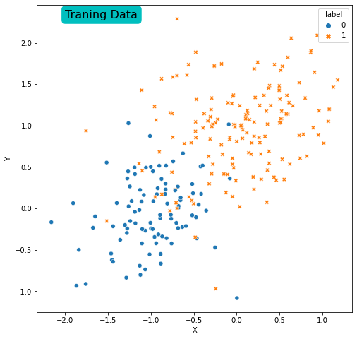
Plot the training and the test data and answer the question that “Are the data linearly separable?”
cols = ['X', 'Y', 'label']
train_ds = pd.read_csv('./hw2_data/classification_trn.txt',
                       delimiter=' +',
                      names=cols,
                      index_col=False,
                      engine='python')
train_ds.shape
(250, 3)
train_ds.head()
| X | Y | label | |
|---|---|---|---|
| 0 | 0.462766 | 0.339111 | 1 |
| 1 | 0.779089 | 0.894436 | 1 |
| 2 | 0.067501 | 0.846257 | 1 |
| 3 | -0.048451 | 0.142165 | 1 |
| 4 | -0.529524 | 0.792441 | 1 |
cols = ['X', 'Y', 'label']
test_ds = pd.read_csv('./hw2_data/classification_tst.txt',
                       delimiter=' +',
                      names=cols,
                      index_col=False,
                      engine='python')
test_ds.shape
(100, 3)
## plotting the training data
plt.figure(figsize=(8,8))
sns.scatterplot(data=train_ds, x='X', y='Y',
                style='label',
                hue='label')
plt.text(y=2.3, x=-2, s='Traning Data', size=16, bbox=dict(boxstyle='round',
                                                          color='c'))
plt.show()
## plotting the test data
plt.figure(figsize=(8,8))
sns.scatterplot(data=test_ds, x='X', y='Y',
                style='label',
                hue='label')
plt.text(y=2, x=-0.5, s='Test Data', size=16, bbox=dict(boxstyle='round',
                                                          color='c'))
plt.show()
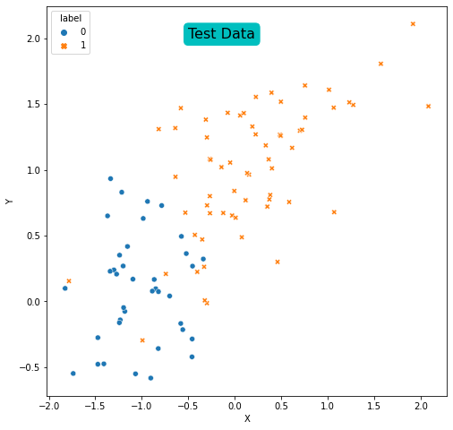
It is possible to see that the data is not linearly separable in training set.
P2, P3, P4#
Question: Find the gradient descent formulas in order to maximize the likelihood of the regression and using the initial weights as \(1\) apply the learning rate \(\frac{1}{t}\). (\(t\) is the time steps \(1, 2, ..., T\))
\begin{equation} W^{new} \leftarrow W^{old} + \alpha(i)\sum_{i=1}^{n} \big( y_i - f(x_i, W^{old})\big) x_{i} \ \text{Where }\alpha(i) = \frac{1}{i} \text{ For i=1, 2, …} \end{equation}
The learning_rate=0 corresponds to \(\frac{2}{t}\) and the learning_rate=1 corresponds to \(\frac{1}{\sqrt{t}}\).
Also the iterations can be adjusted using the argument iterations.
The errors are plotted in images that are saved within the HW2 folder.
!python3 scripts/main2_5.py learning_rate=0 iterations=500
Logistic Regression on housing dataset!
----------------------------------------------------------------------
----------------------------------------------------------------------
Loading Training and Test sets
datasets loaded!
Train set head:
          X         Y
0  0.462766  0.339111
1  0.779089  0.894436
2  0.067501  0.846257
3 -0.048451  0.142165
4 -0.529524  0.792441
Test set head :
          X         Y
0 -0.521659  0.363769
1 -0.993098 -0.295949
2  2.083345  1.483410
3 -0.866462  0.166879
4 -1.182918 -0.075403
----------------------------------------------------------------------
----------------------------------------------------------------------
Closed Form Training:
 Train Error:
  Mean Squared Error: 0.18533821040260134
 Test Error:
  0.28
 Final Weights of the closed form training
[-0.10041674  0.74624728]
----------------------------------------------------------------------
----------------------------------------------------------------------
Gradient descent For Logistic Regression with T=500 iterations
 Train Errors:
  MSE: [21.179730570075883]
 Test Error:
  MSE: 7.0

 Final wights of Offline Gradient Descent Learning
[[2.66828095]
 [2.44634553]]
----------------------------------------------------------------------
----------------------------------------------------------------------
Incremental Learning (Online GD)
  Training Error:
   MSE:[[0.7290789712448449, 0.07]]
  Test Error:
   MSE:0.07

 Final wights of Incremental Learning
[4.0564108  3.72600682]
----------------------------------------------------------------------
P5#
The learning rate is \(\frac{1}{t}\) in the cell below
!python3 scripts/main2_5.py learning_rate=1 iterations=500
Logistic Regression on housing dataset!
----------------------------------------------------------------------
----------------------------------------------------------------------
Loading Training and Test sets
datasets loaded!
Train set head:
          X         Y
0  0.462766  0.339111
1  0.779089  0.894436
2  0.067501  0.846257
3 -0.048451  0.142165
4 -0.529524  0.792441
Test set head :
          X         Y
0 -0.521659  0.363769
1 -0.993098 -0.295949
2  2.083345  1.483410
3 -0.866462  0.166879
4 -1.182918 -0.075403
----------------------------------------------------------------------
----------------------------------------------------------------------
Closed Form Training:
 Train Error:
  Mean Squared Error: 0.18533821040260134
 Test Error:
  0.28
 Final Weights of the closed form training
[-0.10041674  0.74624728]
----------------------------------------------------------------------
----------------------------------------------------------------------
Gradient descent For Logistic Regression with T=500 iterations
 Train Errors:
  MSE: [21.514205312276683]
 Test Error:
  MSE: 7.0

 Final wights of Offline Gradient Descent Learning
[[3.81875707]
 [3.33814397]]
----------------------------------------------------------------------
----------------------------------------------------------------------
Incremental Learning (Online GD)
  Training Error:
   MSE:[[0.7268892378981953, 0.07]]
  Test Error:
   MSE:0.07

 Final wights of Incremental Learning
[13.60834642 14.01209199]
----------------------------------------------------------------------
And using static learning rate 0.5 in below
!python3 scripts/main2_5.py learning_rate=0.5 iterations=500
Logistic Regression on housing dataset!
----------------------------------------------------------------------
----------------------------------------------------------------------
Loading Training and Test sets
datasets loaded!
Train set head:
          X         Y
0  0.462766  0.339111
1  0.779089  0.894436
2  0.067501  0.846257
3 -0.048451  0.142165
4 -0.529524  0.792441
Test set head :
          X         Y
0 -0.521659  0.363769
1 -0.993098 -0.295949
2  2.083345  1.483410
3 -0.866462  0.166879
4 -1.182918 -0.075403
----------------------------------------------------------------------
----------------------------------------------------------------------
Closed Form Training:
 Train Error:
  Mean Squared Error: 0.18533821040260134
 Test Error:
  0.28
 Final Weights of the closed form training
[-0.10041674  0.74624728]
----------------------------------------------------------------------
----------------------------------------------------------------------
Gradient descent For Logistic Regression with T=500 iterations
 Train Errors:
  MSE: [22.45222254661859]
 Test Error:
  MSE: 8.0

 Final wights of Offline Gradient Descent Learning
[[6.0130267 ]
 [4.98060682]]
----------------------------------------------------------------------
----------------------------------------------------------------------
Incremental Learning (Online GD)
  Training Error:
   MSE:[[0.7357933632670419, 0.07]]
  Test Error:
   MSE:0.07

 Final wights of Incremental Learning
[75.46032218 77.3744382 ]
----------------------------------------------------------------------
In high iteration counts there is no obvious difference between different learning rates (But it just seems the \(\frac{2}{t}\) learning rate is doing better). To find the difference we used 50 iterations in below
!python3 scripts/main2_5.py learning_rate=0 iterations=50
Logistic Regression on housing dataset!
----------------------------------------------------------------------
----------------------------------------------------------------------
Loading Training and Test sets
datasets loaded!
Train set head:
          X         Y
0  0.462766  0.339111
1  0.779089  0.894436
2  0.067501  0.846257
3 -0.048451  0.142165
4 -0.529524  0.792441
Test set head :
          X         Y
0 -0.521659  0.363769
1 -0.993098 -0.295949
2  2.083345  1.483410
3 -0.866462  0.166879
4 -1.182918 -0.075403
----------------------------------------------------------------------
----------------------------------------------------------------------
Closed Form Training:
 Train Error:
  Mean Squared Error: 0.18533821040260134
 Test Error:
  0.28
 Final Weights of the closed form training
[-0.10041674  0.74624728]
----------------------------------------------------------------------
----------------------------------------------------------------------
Gradient descent For Logistic Regression with T=50 iterations
 Train Errors:
  MSE: [21.321777405908414]
 Test Error:
  MSE: 7.0

 Final wights of Offline Gradient Descent Learning
[[2.34004787]
 [2.17965517]]
----------------------------------------------------------------------
----------------------------------------------------------------------
Incremental Learning (Online GD)
  Training Error:
   MSE:[[0.743316177460033, 0.07]]
  Test Error:
   MSE:0.07

 Final wights of Incremental Learning
[2.70364651 2.3125385 ]
----------------------------------------------------------------------
!python3 scripts/main2_5.py learning_rate=1 iterations=50
Logistic Regression on housing dataset!
----------------------------------------------------------------------
----------------------------------------------------------------------
Loading Training and Test sets
datasets loaded!
Train set head:
          X         Y
0  0.462766  0.339111
1  0.779089  0.894436
2  0.067501  0.846257
3 -0.048451  0.142165
4 -0.529524  0.792441
Test set head :
          X         Y
0 -0.521659  0.363769
1 -0.993098 -0.295949
2  2.083345  1.483410
3 -0.866462  0.166879
4 -1.182918 -0.075403
----------------------------------------------------------------------
----------------------------------------------------------------------
Closed Form Training:
 Train Error:
  Mean Squared Error: 0.18533821040260134
 Test Error:
  0.28
 Final Weights of the closed form training
[-0.10041674  0.74624728]
----------------------------------------------------------------------
----------------------------------------------------------------------
Gradient descent For Logistic Regression with T=50 iterations
 Train Errors:
  MSE: [21.222015553883374]
 Test Error:
  MSE: 7.0

 Final wights of Offline Gradient Descent Learning
[[2.59108759]
 [2.37625462]]
----------------------------------------------------------------------
----------------------------------------------------------------------
Incremental Learning (Online GD)
  Training Error:
   MSE:[[0.7267833093158856, 0.09]]
  Test Error:
   MSE:0.09

 Final wights of Incremental Learning
[4.70243878 5.20285994]
----------------------------------------------------------------------
## And static learning rate
!python3 scripts/main2_5.py learning_rate=0.5 iterations=500
Logistic Regression on housing dataset!
----------------------------------------------------------------------
----------------------------------------------------------------------
Loading Training and Test sets
datasets loaded!
Train set head:
          X         Y
0  0.462766  0.339111
1  0.779089  0.894436
2  0.067501  0.846257
3 -0.048451  0.142165
4 -0.529524  0.792441
Test set head :
          X         Y
0 -0.521659  0.363769
1 -0.993098 -0.295949
2  2.083345  1.483410
3 -0.866462  0.166879
4 -1.182918 -0.075403
----------------------------------------------------------------------
----------------------------------------------------------------------
Closed Form Training:
 Train Error:
  Mean Squared Error: 0.18533821040260134
 Test Error:
  0.28
 Final Weights of the closed form training
[-0.10041674  0.74624728]
----------------------------------------------------------------------
----------------------------------------------------------------------
Gradient descent For Logistic Regression with T=500 iterations
 Train Errors:
  MSE: [22.45222254661859]
 Test Error:
  MSE: 8.0

 Final wights of Offline Gradient Descent Learning
[[6.0130267 ]
 [4.98060682]]
----------------------------------------------------------------------
----------------------------------------------------------------------
Incremental Learning (Online GD)
  Training Error:
   MSE:[[0.7357933632670419, 0.07]]
  Test Error:
   MSE:0.07

 Final wights of Incremental Learning
[75.46032218 77.3744382 ]
----------------------------------------------------------------------
We lower the iteration counts more to see better the differences
!python3 scripts/main2_5.py learning_rate=0 iterations=5
Logistic Regression on housing dataset!
----------------------------------------------------------------------
----------------------------------------------------------------------
Loading Training and Test sets
datasets loaded!
Train set head:
          X         Y
0  0.462766  0.339111
1  0.779089  0.894436
2  0.067501  0.846257
3 -0.048451  0.142165
4 -0.529524  0.792441
Test set head :
          X         Y
0 -0.521659  0.363769
1 -0.993098 -0.295949
2  2.083345  1.483410
3 -0.866462  0.166879
4 -1.182918 -0.075403
----------------------------------------------------------------------
----------------------------------------------------------------------
Closed Form Training:
 Train Error:
  Mean Squared Error: 0.18533821040260134
 Test Error:
  0.28
 Final Weights of the closed form training
[-0.10041674  0.74624728]
----------------------------------------------------------------------
----------------------------------------------------------------------
Gradient descent For Logistic Regression with T=5 iterations
 Train Errors:
  MSE: [21.954185815907675]
 Test Error:
  MSE: 7.0

 Final wights of Offline Gradient Descent Learning
[[1.90462057]
 [1.81567883]]
----------------------------------------------------------------------
----------------------------------------------------------------------
Incremental Learning (Online GD)
  Training Error:
   MSE:[[1.0534808105827163, 0.32000000000000006]]
  Test Error:
   MSE:0.32000000000000006

 Final wights of Incremental Learning
[ 0.82746549 -0.11811742]
----------------------------------------------------------------------
!python3 scripts/main2_5.py learning_rate=1 iterations=5
Logistic Regression on housing dataset!
----------------------------------------------------------------------
----------------------------------------------------------------------
Loading Training and Test sets
datasets loaded!
Train set head:
          X         Y
0  0.462766  0.339111
1  0.779089  0.894436
2  0.067501  0.846257
3 -0.048451  0.142165
4 -0.529524  0.792441
Test set head :
          X         Y
0 -0.521659  0.363769
1 -0.993098 -0.295949
2  2.083345  1.483410
3 -0.866462  0.166879
4 -1.182918 -0.075403
----------------------------------------------------------------------
----------------------------------------------------------------------
Closed Form Training:
 Train Error:
  Mean Squared Error: 0.18533821040260134
 Test Error:
  0.28
 Final Weights of the closed form training
[-0.10041674  0.74624728]
----------------------------------------------------------------------
----------------------------------------------------------------------
Gradient descent For Logistic Regression with T=5 iterations
 Train Errors:
  MSE: [22.70260229673039]
 Test Error:
  MSE: 7.0

 Final wights of Offline Gradient Descent Learning
[[1.6710624 ]
 [1.60624242]]
----------------------------------------------------------------------
----------------------------------------------------------------------
Incremental Learning (Online GD)
  Training Error:
   MSE:[[1.0748037987641088, 0.28]]
  Test Error:
   MSE:0.28

 Final wights of Incremental Learning
[ 0.5997547  -0.00995924]
----------------------------------------------------------------------
!python3 scripts/main2_5.py learning_rate=0.5 iterations=5
Logistic Regression on housing dataset!
----------------------------------------------------------------------
----------------------------------------------------------------------
Loading Training and Test sets
datasets loaded!
Train set head:
          X         Y
0  0.462766  0.339111
1  0.779089  0.894436
2  0.067501  0.846257
3 -0.048451  0.142165
4 -0.529524  0.792441
Test set head :
          X         Y
0 -0.521659  0.363769
1 -0.993098 -0.295949
2  2.083345  1.483410
3 -0.866462  0.166879
4 -1.182918 -0.075403
----------------------------------------------------------------------
----------------------------------------------------------------------
Closed Form Training:
 Train Error:
  Mean Squared Error: 0.18533821040260134
 Test Error:
  0.28
 Final Weights of the closed form training
[-0.10041674  0.74624728]
----------------------------------------------------------------------
----------------------------------------------------------------------
Gradient descent For Logistic Regression with T=5 iterations
 Train Errors:
  MSE: [23.278982955755232]
 Test Error:
  MSE: 7.0

 Final wights of Offline Gradient Descent Learning
[[1.54112266]
 [1.4904238 ]]
----------------------------------------------------------------------
----------------------------------------------------------------------
Incremental Learning (Online GD)
  Training Error:
   MSE:[[1.1067532327276703, 0.23]]
  Test Error:
   MSE:0.23

 Final wights of Incremental Learning
[0.42850402 0.02784965]
----------------------------------------------------------------------
In the results we can see that there may be a little difference and the static learning rate 0.5 show the better results on Test Error in Incremental learning Gradient Descent.
P6#
Comparing the Incremental version of logisitic regression with the normal version shows that it can achive better results with high iteration counts.
Q5#
The data is used from the question 4 and Nive bayes method will be applied.
def probability_normal_distribution(X, mu, sigma):
    """
    The probability value for normal distribution function

    Parameters:
    ------------
    x : array_like
        the input data
    mu : float
        the mean value given
    sigma : float
        the variance given

    Returns:
    --------
    probability : float
        the probability value for the x input values
    """
    ## we've divided the equation in two parts
    p1 = 1 / (np.sqrt(np.pi * 2) * sigma)
    p2 = np.exp(-0.5 * ((X-mu) / sigma)**2 )

    probability = p1 * p2

    return probability

def find_MLE_Normal_distro(X):
    """
    the maximum likelihood estimation for parameters of normal distribution
    the parameters for normal distribution is covariance matrix and mean vector

    Parameters:
    ------------
    X : array_like
        the X input data vectors

    Returns:
    ---------
    mu : array_like
        the means vector
    variance : matrix_like
        the matrix representing the covariance

    """
    X = np.array(X)

    mu = (1 / len(X)) * np.sum(X)

    ## some changes was made to the ML estimation of variance
    ## because of dataset shape
    variance = np.sqrt((1 / len(X)) * np.sum((X - mu)**2))

    return mu, variance
cols = ['X', 'Y', 'label']
train_ds = pd.read_csv('./hw2_data/classification_trn.txt',
                       delimiter=' +',
                      names=cols,
                      index_col=False,
                      engine='python')

test_ds = pd.read_csv('./hw2_data/classification_tst.txt',
                       delimiter=' +',
                      names=cols,
                      index_col=False,
                      engine='python')
In Naive Bayes the class conditional density can be computed by \begin{equation} p(x|c=1) = \prod_{i=1}^{d} p(x_i | c=1) \ p(x|c=0) = \prod_{i=1}^{d} p(x_i | c=0) \end{equation}
## divide the dataset into 0 and 1 labels
def estimate_MLE_NB(X, Y, features_arr):
    """
    estimate the Maximum likelihood parameters for naive bayes method
    in detail: in naive bayes we have a parameter for each dimension and each class

    Parameters:
    ------------
    X : array_like
        the input data (a pandas dataframe is prefered)
    Y : array_like
        the labels for each `X` inputs
    features : array_like
        the string array for the name of each label in training data (dimensions)

    Returns:
    --------
    MLE_estimates : dictionary
        the estimated parameters as a dictionary
    """
    ## dictionary of maximum likelihood estimations
    MLE_estimates = {}
    for feature in features_arr:
        for label in [0, 1]:
            mu, var = find_MLE_Normal_distro(X[Y == label][feature])
            ## each feature of class estimation
            MLE_estimates[f'{feature},{label}'] = [mu, var]
    return MLE_estimates
##################### Code is Implemented in the function above #####################

# ## dictionary of maximum likelihood estimations
# MLE_estimates = {}
# for feature in ['X', 'Y']:
#     for label in [0, 1]:
#         mu, var = find_MLE_Normal_distro(train_ds[train_ds.label == label][feature])
#         ## each feature of class estimation
#         MLE_estimates[f'{feature},{label}'] = [mu, var]


MLE_estimates = estimate_MLE_NB(train_ds[['X', 'Y']], train_ds[['label']].values, ['X', 'Y'])
MLE_estimates
{'X,0': [-0.9766294551726316, 0.4043628347745132],
 'X,1': [0.01564038684774194, 0.574343819845795],
 'Y,0': [-0.04355836269157895, 0.42688761701060846],
 'Y,1': [0.9415618305584516, 0.5324787748723679]}
def predict_NB(X, MLE_estimations, features_arr):
    """
    predict the class Using Naive bayes algorithm

    Parameters:
    ------------
    X : pandas dataframe
        Input data, `X` and `Y` should be the features
    MLE_estimations : dictionary
        Maximum likelihood estimations corresponding to each dimension and class as a dictionary with keys like `X,0`
        meaning X as first feature and 0 as first class

    Returns:
    ---------
    prediction : array_like
        the array representing the probability of each class for data
    """
    ## the predicted value for each data
    prediction = []
    for idx in range(len(X)):
        ## initialize Class probability array
        class_p_arr = []
        for i in [0, 1]:
            ## multiply probability for each dimension
            p = 1
            for feature in features_arr:
                mu, var = MLE_estimations[f'{feature},{i}']
                p = p * probability_normal_distribution(X.iloc[idx][feature],mu, var)
            class_p_arr.append(p)
        ## save each class probability of each data
        prediction.append(class_p_arr)

    ## for ease of use convert to numpy
    prediction = np.array(prediction)
    return prediction
results  = predict_NB(train_ds[['X', 'Y']], MLE_estimates, ['X', 'Y'])
results.shape
(250, 2)
results[:4]
array([[1.09327234e-03, 2.02663171e-01],
       [6.64630522e-06, 2.14271447e-01],
       [3.74476058e-03, 5.10057518e-01],
       [6.01875199e-02, 1.67582766e-01]])
y_pred = (results[:, 0] < results[:, 1]).astype(int)
## Accuracy
(y_pred == train_ds[['label']].T.values).sum() / len(y_pred)
0.9
def probability_multivariate_normal_distribution(X,mu, sigma):
"""
The probability value for multivariate normal distribution function
Parameters:
------------
x : array_like
the input data
mu : array_like
the means vector
sigma : matrix_like
the matrix representing the covariance
Returns:
--------
probability : float
the probability value for the x input values
"""
dimension = len(mu)
## divide the formula into 2 parts
p1 = 1 / np.sqrt(((2*np.pi)**dimension) * np.linalg.det(sigma))
## some changes was made to the equation
## because of dataset shape
p2 = np.exp(-1/2 * (np.dot(X-mu, np.linalg.inv(sigma) @ (X-mu).T)))
probability = p1 * p2
return probability
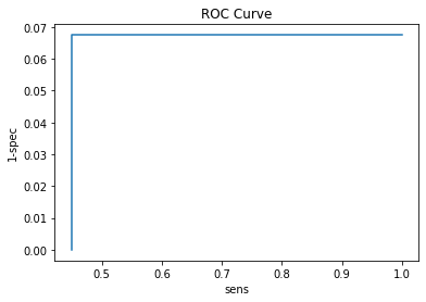
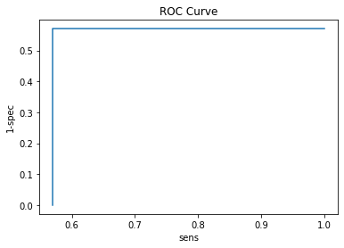
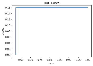
def roc_curve(y, y_pred):
"""
draw the roc curve
Parameters:
------------
y : array_like
the actual output for the data
y_pred : array_like
the predicted output for data
"""
scores = []
## find the values for each threshold
## TP -> True Positive
## TN -> True Negative
## FP -> False Positive
## FN -> False Negative
for threshold in np.linspace(0, 1, 101):
TP = ((y_pred >= threshold) & (y == 1)).sum()
TN = ((y_pred <= threshold) & (y == 0)).sum()
FP = ((y_pred > threshold) & (y == 0)).sum()
FN = ((y_pred < threshold) & (y == 1)).sum()
scores.append([threshold, TP, TN, FP, FN])
df_cols = ['threshold', 'TP', 'TN', 'FP', 'FN']
df_scores = pd.DataFrame(scores, columns=df_cols)
## sensitivity and specificity
## True Positive rate = sensitivity
df_scores['sens'] = df_scores.TP / (df_scores.TP + df_scores.FN)
## False Positive rate = 1 - specificity
df_scores['1-spec'] = df_scores.FP / (df_scores.FP + df_scores.TN)
plt.plot(df_scores['sens'], df_scores['1-spec'])
plt.xlabel('sens')
plt.ylabel('1-spec')
plt.title(f'ROC Curve')
plt.show()
roc_curve(train_ds[['label']].values, y_pred)
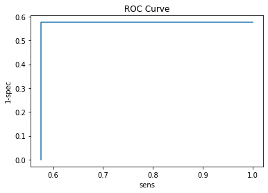
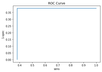
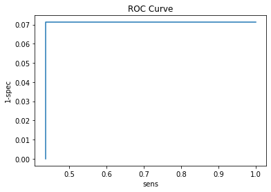
Now we’re going to apply the estimations on test set.
## test set
results = predict_NB(test_ds[['X', 'Y']], MLE_estimates, ['X', 'Y'])
y_pred = (results[:, 0] < results[:, 1]).astype(int)
## test accuracy
(y_pred == test_ds[['label']].T.values).sum() / len(y_pred)
0.91
roc_curve(test_ds[['label']].values, y_pred)
Q6#
Use Quadratic Discriminant Analysis for classification data. The functions for question 5 can be used.
## we need to find the mean and covariance of each class

## divide into class 0 and class 1
train_ds_C0 = train_ds[train_ds.label == 0]
train_ds_C1 = train_ds[train_ds.label == 1]

train_ds_C0_X = train_ds_C0[['X', 'Y']]
train_ds_C0_Y = train_ds_C0[['label']]

train_ds_C1_X = train_ds_C1[['X', 'Y']]
train_ds_C1_Y = train_ds_C1[['label']]

mu0, sigma0 = find_MLE_Normal_distro(train_ds_C0_X.T)
mu1, sigma1 = find_MLE_Normal_distro(train_ds_C1_X.T)
## take a look at properties found
print("Class 0")
print(f'Covariance:\n{sigma0}\nMean vector:\n{mu0}\n')
print('--'*10)
print("Class 1")
print(f'Covariance:\n{sigma1}\nMean vector:\n{mu1}\n')
Class 0
Covariance:
467.38705057468275
Mean vector:
-48.45892134854999

--------------------
Class 1
Covariance:
917.6585102015431
Mean vector:
74.18317184898
Implementing The functions above and some other in a Class.
class QDA():
    """
    Quadratic Discriminant Analysis Class
    """
    def __init__(self):
        self.mu0 = None
        self.mu1 = None
        self.sigma0 = None
        self.sigma1 = None

    __
    def predict(self, X):
        """
        Predict the output for the X input

        Parameters:
        ------------
        X : array_like
            The data to be appended
        """
        mu0 = self.mu0
        mu1 = self.mu1
        sigma0 = self.sigma0
        sigma1 = self.sigma1

        ## check if the model is not learned and the parameters is updated
        ## checking one parameter is enough
        ## because we are assigning a value to all in learning phase
        if len(sigma0) == 0:
            raise "Error! First fit the model on a dataset then try to predict the values!"


        ## Find the probabilities for class 0
        ## save them in an array for furthur comparisons
        prediction = []
        for i in range(len(X)):
            ## Find the predicted Class of each data in class 0
            P_Class0 = self.__probability_multivariate_normal_distribution(X.iloc[i]
                                                             ,mu0, sigma0)

            P_Class1 = self.__probability_multivariate_normal_distribution(X.iloc[i]
                                                             ,mu1, sigma1)
            ## Compare and set the class to highest probability
            P = P_Class1 >= P_Class0

            ## Append the number of Class
            prediction.append(int(P))

        return prediction
    def fit(self, X):
        """
        Learning the parameters of the model (Binary Classification model!)

        Parameters:
        -----------
        X : array_like (pandas dataframe is preferred)
            the input values to be learned, With outputs as label
        # Y : array_like
        #     the label for the data (The binary classification task is here)
        """
        ## we need to find the mean and covariance of each class

        features_arr = X.columns[:-1]

        ## divide into class 0 and class 1
        train_ds_C0 = X[X.label == 0]
        train_ds_C1 = X[X.label == 1]

        # train_ds_C0_X = train_ds_C0[['X', 'Y']]
        train_ds_C0_X = train_ds_C0[features_arr]

        # train_ds_C0_Y = train_ds_C0[['label']]

        train_ds_C1_X = train_ds_C1[features_arr]
        # train_ds_C1_Y = train_ds_C1[['label']]

        mu0, sigma0 = self.__find_MLE_Normal_distro(train_ds_C0_X.T)
        mu1, sigma1 = self.__find_MLE_Normal_distro(train_ds_C1_X.T)

        ## Save the parameters of the model
        self.mu0 = mu0
        self.mu1 = mu1
        self.sigma0 = sigma0
        self.sigma1 = sigma1

    def __probability_multivariate_normal_distribution(self, X, mu, sigma):
        """
        The probability value for multivariate normal distribution function

        Parameters:
        ------------
        x : array_like
            the input data
        mu : array_like
            the means vector
        sigma : matrix_like
            the matrix representing the covariance

        Returns:
        --------
        probability : float
            the probability value for the x input values
        """
        dimension = len(mu)

        ## divide the formula into 2 parts
        p1 = 1 / np.sqrt(((2*np.pi)**dimension) * np.linalg.det(sigma))

        ## some changes was made to the equation
        ## because of dataset shape
        p2 = np.exp(-1/2 * (np.dot(X-mu, np.linalg.inv(sigma) @ (X-mu).T)))


        probability = p1 * p2

        return probability

    def __find_MLE_Normal_distro(self, X):
        """
        the maximum likelihood estimation for parameters of multivatiate normal distribution
        the parameters for normal distribution is covariance matrix and mean vector

        Parameters:
        ------------
        X : array_like
            the X input data vectors

        Returns:
        ---------
        mu : array_like
            the means vector
        covariance : matrix_like
            the matrix representing the covariance

        """

        mu = (1 / len(X.T)) * np.sum(X, axis=1)

        ## some changes was made to the ML estimation of covariance
        ## because of dataset shape
        covariance = (1 / len(X.T)) * ((X.T-mu).T @ (X.T-mu))

        return mu, covariance
## convert probabilities to numpy array
model_QDA = QDA()

train_ds_X = train_ds[['X', 'Y']]
train_ds_Y = train_ds[['label']]

model_QDA.fit(train_ds)
test_Y_pred = model_QDA.predict(test_ds[['X','Y']])
train_Y_pred = model_QDA.predict(train_ds_X)
print(f'Mu0:\n{model_QDA.mu0}\n')
print(f'Mu1:\n{model_QDA.mu1}')
Mu0:
X   -0.976629
Y   -0.043558
dtype: float64

Mu1:
X    0.015640
Y    0.941562
dtype: float64
print(f'Covariance_0:\n {model_QDA.sigma0}\n')
print(f'Covariance_1:\n {model_QDA.sigma1}\n')
Covariance_0:
           X         Y
X  0.163509  0.040219
Y  0.040219  0.182233

Covariance_1:
           X         Y
X  0.329871  0.092079
Y  0.092079  0.283534
## test accuracy
test_Y = test_ds[['label']].values.flatten()

acc_test = (test_Y == test_Y_pred).sum() / len(test_Y_pred)
acc_test
0.9
def find_ROC(y_pred, y_true, thresholds = 101):
    """
    Find the confusion matrix for each threshold (ROC)

    Parameters:
    ------------
    y_true : array_like
        the actual output of inputs
    y_pred : array_like
        the predicted values of inputs
    thresholds : positive integer
        the count of thresholds to be evaluated between 0 and 1
        default is 101

    Returns:
    ---------
    df_scores : pandas dataframe
        dataframe contains the confusion matrix for different thresholds
    """

    assert thresholds >= 5, "Error: Thresholds must be more than 5!"

    scores = []

    ## find the values for each threshold
    ## TP -> True Positive
    ## TN -> True Negative
    ## FP -> False Positive
    ## FN -> False Negative
    for threshold in np.linspace(0, 1, thresholds):
        TP = ((y_pred >= threshold) & (y_true == 1)).sum()
        TN = ((y_pred <= threshold) & (y_true == 0)).sum()
        FP = ((y_pred > threshold) & (y_true == 0)).sum()
        FN = ((y_pred < threshold) & (y_true == 1)).sum()


        scores.append([threshold, TP, TN, FP, FN])

    df_cols = ['threshold', 'TP', 'TN', 'FP', 'FN']
    df_scores = pd.DataFrame(scores, columns=df_cols)

    ## sensitivity and specificity
    ## True Positive rate = sensitivity
    df_scores['sens'] = df_scores.TP / (df_scores.TP + df_scores.FN)
    ## False Positive rate = 1 - specificity
    df_scores['1-spec'] = df_scores.FP / (df_scores.FP + df_scores.TN)

    return df_scores
def export_ROC_Curve(df_scores, description):
    """
    save the roc curve using the dataframe scores

    Parameters:
    ------------
    df_scores : array_like
        the results computed for different thresholds
    description : string
        the name of the saved file
    """

    plt.plot(df_scores['sens'], df_scores['1-spec'])
    plt.title(f'ROC Curve for {description}')
    plt.savefig(f'Q6_QDA_{description}.png')
    plt.close()
roc_scores = find_ROC(test_Y_pred, test_Y)
export_ROC_Curve(roc_scores, 'MLE')
roc_scores.iloc[np.linspace(0, 100, 10, dtype=int)]
| threshold | TP | TN | FP | FN | sens | 1-spec | |
|---|---|---|---|---|---|---|---|
| 0 | 0.00 | 62 | 35 | 3 | 0 | 1.000000 | 0.078947 |
| 11 | 0.11 | 55 | 35 | 3 | 7 | 0.887097 | 0.078947 |
| 22 | 0.22 | 55 | 35 | 3 | 7 | 0.887097 | 0.078947 |
| 33 | 0.33 | 55 | 35 | 3 | 7 | 0.887097 | 0.078947 |
| 44 | 0.44 | 55 | 35 | 3 | 7 | 0.887097 | 0.078947 |
| 55 | 0.55 | 55 | 35 | 3 | 7 | 0.887097 | 0.078947 |
| 66 | 0.66 | 55 | 35 | 3 | 7 | 0.887097 | 0.078947 |
| 77 | 0.77 | 55 | 35 | 3 | 7 | 0.887097 | 0.078947 |
| 88 | 0.88 | 55 | 35 | 3 | 7 | 0.887097 | 0.078947 |
| 100 | 1.00 | 55 | 38 | 0 | 7 | 0.887097 | 0.000000 |
Q7#
## column names are used from ```pima-indians-diabetes.name``` file
cols = ['pregnancy_count', 'glucose_test', 'blood_pressure', 'triceps_thickness', '2h_insulin', 'mass', 'pedi', 'age', 'label']

df_pima = pd.read_csv('../HW1/hw1_data/pima/pima-indians-diabetes.data', index_col=False ,names=cols)
df_pima.head()
| pregnancy_count | glucose_test | blood_pressure | triceps_thickness | 2h_insulin | mass | pedi | age | label | |
|---|---|---|---|---|---|---|---|---|---|
| 0 | 6 | 148 | 72 | 35 | 0 | 33.6 | 0.627 | 50 | 1 |
| 1 | 1 | 85 | 66 | 29 | 0 | 26.6 | 0.351 | 31 | 0 |
| 2 | 8 | 183 | 64 | 0 | 0 | 23.3 | 0.672 | 32 | 1 |
| 3 | 1 | 89 | 66 | 23 | 94 | 28.1 | 0.167 | 21 | 0 |
| 4 | 0 | 137 | 40 | 35 | 168 | 43.1 | 2.288 | 33 | 1 |
##################### From HW1 #####################
def divideset2(df, fraction = 0.66):
    """
    Divide the dataset into train and test with fixed size every run

    INPUTS:
    ---------
    df: pandas dataframe, the dataset that is going to be splitted
    fraction: the value to divide the dataset, default is 0.66

    OUTPUTS:
    ---------
    train: pandas dataframe, the portion of the dataset for train
    test: pandas dataframe, the portion of the dataset for test
    """

    train = df.sample(frac=0.66).copy()
    test = df.drop(train.index)

    return train, test
df_pima_trn, df_pima_tst = divideset2(df_pima)
df_pima_trn.shape
(507, 9)
df_pima_tst.shape
(261, 9)
We have modified the script for question 4 and run it here.
!python3 scripts/main_2_7.py
Logistic Regression on housing dataset!
----------------------------------------------------------------------
----------------------------------------------------------------------
Loading Training and Test sets
datasets loaded!
Train set head:
   pregnancy_count  glucose_test  blood_pressure  ...  mass   pedi  age
0                6           148              72  ...  33.6  0.627   50
1                1            85              66  ...  26.6  0.351   31
2                8           183              64  ...  23.3  0.672   32
3                1            89              66  ...  28.1  0.167   21
4                0           137              40  ...  43.1  2.288   33

[5 rows x 8 columns]
----------------------------------------------------------------------
----------------------------------------------------------------------
Closed Form Training:
 Train Error:
  Mean Squared Error: 0.1791001059784589
 Test Error:
  0.6471354166666666
 Final Weights of the closed form training
[ 2.46554784e-02  3.86639820e-03 -4.91162585e-03  5.75161548e-05
  4.78331990e-05  4.18631699e-03  9.80129310e-02 -1.04267995e-03]
----------------------------------------------------------------------
----------------------------------------------------------------------
Gradient descent For Logistic Regression with T=50 iterations
 Train Errors:
scripts/main_2_7.py:148: RuntimeWarning: overflow encountered in exp
  y = 1 / (1 + np.exp(-w.T @ x))
  MSE: [395.00014894191975]
 Test Error:
  MSE: 395.0

 Final wights of Offline Gradient Descent Learning
[[ -12.22417034]
 [  50.06305025]
 [ -46.92348329]
 [  77.92385392]
 [  17.51867599]
 [-122.31863815]
 [   7.4775007 ]
 [  -0.72949004]]
----------------------------------------------------------------------
----------------------------------------------------------------------
Incremental Learning (Online GD)
  Training Error:
   MSE:[[1.0178211994736963, 0.6510416666666666]]
  Test Error:
   MSE:0.6510416666666666

 Final wights of Incremental Learning
[0.80728208 3.19264994 0.06047742 2.39362356 0.54607482 0.85250314
 1.88412344 2.44401855]
----------------------------------------------------------------------
Q8#
Use Naive bayes implemented and used by question 5 for pima dataset.
pima_cols_X = df_pima_trn.columns[:-1]
MLE_estimates_Q8 = estimate_MLE_NB(df_pima_trn[pima_cols_X], df_pima_trn[['label']].values, pima_cols_X )
MLE_estimates_Q8
{'pregnancy_count,0': [3.3827893175074184, 3.075518425354172],
 'pregnancy_count,1': [4.947058823529412, 3.5616614839076943],
 'glucose_test,0': [109.9406528189911, 26.209089248154815],
 'glucose_test,1': [140.91764705882352, 33.11715807809526],
 'blood_pressure,0': [68.31750741839762, 18.76743713077681],
 'blood_pressure,1': [69.69411764705882, 21.696312253420487],
 'triceps_thickness,0': [19.762611275964392, 15.091512038708125],
 'triceps_thickness,1': [22.605882352941176, 17.416455051886835],
 '2h_insulin,0': [65.35311572700297, 91.42289286036038],
 '2h_insulin,1': [103.74705882352941, 139.6904166052542],
 'mass,0': [30.332640949554893, 7.0884075860170555],
 'mass,1': [34.94529411764706, 6.658175529684017],
 'pedi,0': [0.4379050445103858, 0.30617648254103347],
 'pedi,1': [0.5496176470588235, 0.3501867917274237],
 'age,0': [31.42433234421365, 11.96313829923815],
 'age,1': [36.67058823529412, 10.740126229178365]}
results_Q8 = predict_NB(df_pima_trn[pima_cols_X], MLE_estimates_Q8, pima_cols_X)
results_Q8.shape
(507, 2)
training set accuracy
y_pred = (results_Q8[:, 0] < results_Q8[:, 1]).astype(int)
## Accuracy
(y_pred == df_pima_trn[['label']].T.values).sum() / len(y_pred)
0.757396449704142
Training ROC
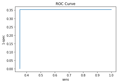
roc_curve(df_pima_trn[['label']].values, y_pred)
Test accuracy and ROC curve
results_Q8_tst = predict_NB(df_pima_tst[pima_cols_X], MLE_estimates_Q8, pima_cols_X)
y_pred = (results_Q8_tst[:, 0] < results_Q8_tst[:, 1]).astype(int)
## Accuracy
(y_pred == df_pima_tst[['label']].T.values).sum() / len(y_pred)
0.7624521072796935
roc_curve(df_pima_tst[['label']].values, y_pred)
Q9#
Use QDA implemented in question 6 for pima dataset.
mode_QDA_pima = QDA()
## the dataframe with the output value will be sent
## the output column is named 'label'
mode_QDA_pima.fit(df_pima_trn)
results_Q9 = mode_QDA_pima.predict(df_pima_trn[pima_cols_X])
## accuracy
(results_Q9 == df_pima_trn[['label']].T.values).sum() / len(results_Q9)
0.7554240631163708
results_Q9 = np.array(results_Q9)

roc_curve(df_pima_trn[['label']].values.flatten(), results_Q9 )
Let’s take a look at the test set.
results_Q9_tst = mode_QDA_pima.predict(df_pima_tst[pima_cols_X])
## accuracy
(results_Q9_tst == df_pima_tst[['label']].T.values).sum() / len(results_Q9_tst)
0.7586206896551724
## ROC curve
results_Q9 = np.array(results_Q9)

roc_curve(df_pima_tst[['label']].values.flatten(), results_Q9_tst )
Q10#
Use SVM method to predict the outputs of pima dataset.
from sklearn.svm import SVC
model_svm = SVC()

model_svm.fit(df_pima_trn[pima_cols_X], df_pima_trn[['label']].values.flatten())
SVC()
results_Q10 = model_svm.predict(df_pima_trn[pima_cols_X])
## Training Accuracy
(results_Q10 == df_pima_trn[['label']].values.flatten()).sum() / len(results_Q10)
0.7633136094674556
results_Q10_tst = model_svm.predict(df_pima_tst[pima_cols_X])
## Test accuracy
(results_Q10_tst == df_pima_tst[['label']].values.flatten()).sum() / len(results_Q10_tst)
0.7509578544061303
## Train ROC curve
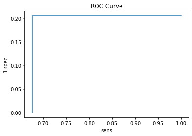
roc_curve(df_pima_trn[['label']].values.flatten(), results_Q10)
## Test ROC curve
roc_curve(df_pima_tst[['label']].values.flatten(), results_Q10_tst)